MMS Hot Plasma Composition Analyzer: Difference between revisions
(adding hpca page) |
No edit summary |
||
| (9 intermediate revisions by the same user not shown) | |||
| Line 3: | Line 3: | ||
The MMS HPCA measures the distribution of hydrogen, helium, and oxygen ions using an electrostatic analyzer. SPEDAS provides command line and [[GUI]] access to HPCA data. | The MMS HPCA measures the distribution of hydrogen, helium, and oxygen ions using an electrostatic analyzer. SPEDAS provides command line and [[GUI]] access to HPCA data. | ||
For more information on the HPCA instrument, please see the HPCA Data Products Guide: | |||
https://lasp.colorado.edu/ | https://lasp.colorado.edu/mms/sdc/public/datasets/hpca/ ([https://lasp.colorado.edu/mms/sdc/public/datasets/hpca/10160.13-MMS-HPCA_SCI_ALG_UM_20160310_0.pdf 10160.13 MMS HPCA SCI ALG UM 20160310]) | ||
For basic command line access see: | For basic command line access see: | ||
<div style="border: 1px solid LightGray; background-color:#F9F9F9; padding: 2px 10px; margin-left: 5px; overflow:hidden;"> | <div style="border: 1px solid LightGray; background-color:#F9F9F9; padding: 2px 10px; margin-left: 5px; overflow:hidden;"> | ||
/projects/ | /projects/mms/examples/basic/mms_load_hpca_crib.pro | ||
/projects/ | /projects/mms/examples/basic/mms_load_hpca_burst_crib.pro | ||
</div> | </div> | ||
| Line 23: | Line 23: | ||
To load and plot HPCA moments for MMS1 on March 7, 2016: | To load and plot HPCA moments for MMS1 on March 7, 2016: | ||
< | <syntaxhighlight lang="idl"> | ||
MMS> mms_load_hpca, probes='1', trange=['2015-10-16', '2015-10-17'], | MMS> mms_load_hpca, probes='1', trange=['2015-10-16', '2015-10-17'], datatype='moments' | ||
MMS> tplot, ['mms1_hpca_hplus_number_density', 'mms1_hpca_oplus_scalar_temperature', 'mms1_hpca_heplus_ion_bulk_velocity'] | MMS> tplot, ['mms1_hpca_hplus_number_density', 'mms1_hpca_oplus_scalar_temperature', 'mms1_hpca_heplus_ion_bulk_velocity'] | ||
</ | </syntaxhighlight> | ||
| Line 37: | Line 37: | ||
To load and plot HPCA energy spectrograms for MMS1 on March 7, 2016: | To load and plot HPCA energy spectrograms for MMS1 on March 7, 2016: | ||
< | <syntaxhighlight lang="idl"> | ||
MMS> mms_load_hpca, probes='1', trange=['2015-10-16', '2015-10-17'], | MMS> mms_load_hpca, probes='1', trange=['2015-10-16', '2015-10-17'], datatype='ion' | ||
MMS> mms_hpca_calc_anodes, fov=[0, 360], probe='1' | MMS> mms_hpca_calc_anodes, fov=[0, 360], probe='1' | ||
MMS> tplot, ['mms1_hpca_hplus_flux_elev_0-360', 'mms1_hpca_oplus_flux_elev_0-360', 'mms1_hpca_heplus_flux_elev_0-360', 'mms1_hpca_heplusplus_flux_elev_0-360'] | MMS> tplot, ['mms1_hpca_hplus_flux_elev_0-360', 'mms1_hpca_oplus_flux_elev_0-360', 'mms1_hpca_heplus_flux_elev_0-360', 'mms1_hpca_heplusplus_flux_elev_0-360'] | ||
</ | </syntaxhighlight> | ||
==SPEDAS derived products== | ==SPEDAS derived products== | ||
[[File: hpca_spd_moments.png |200px|right|HPCA H+ density, velocity, and pressure tensor]] | [[File: hpca_spd_moments.png |200px|right|HPCA H+ density, velocity, and pressure tensor]] | ||
[[File: hpca_spd_spec.png |200px|right|HPCA ]] | [[File: hpca_spd_spec.png |200px|right|HPCA ]] | ||
| Line 60: | Line 58: | ||
<div style="border: 1px solid LightGray; background-color:#F9F9F9; padding: 2px 10px; margin-left: 5px; overflow:hidden;"> | <div style="border: 1px solid LightGray; background-color:#F9F9F9; padding: 2px 10px; margin-left: 5px; overflow:hidden;"> | ||
/projects/ | /projects/mms/examples/advanced/mms_part_products_crib.pro | ||
</div> | </div> | ||
| Line 69: | Line 67: | ||
=== | ===Spectrograms=== | ||
Angular spectrograms are calculated in spacecraft and field-aligned coordinates. Phi (azimuth) and theta (elevation) spectra are calculated in spacecraft coordinates. Gyrophase (azimuth) and pitch angle (co-lat) spectra are calculated in field-aligned coordinates. Magnetic field and ephemeris data are specified via supplementary tplot variables. Energy spectrograms are also available. | Angular spectrograms are calculated in spacecraft and field-aligned coordinates. Phi (azimuth) and theta (elevation) spectra are calculated in spacecraft coordinates. Gyrophase (azimuth) and pitch angle (co-lat) spectra are calculated in field-aligned coordinates. Magnetic field and ephemeris data are specified via supplementary tplot variables. Energy spectrograms are also available. | ||
| Line 76: | Line 74: | ||
===2D slices=== | ===2D slices=== | ||
Slices of full 3D particle data can be visualized as smooth contours or by angle/energy bin. | Slices of full 3D particle data can be visualized as smooth contours or by angle/energy bin. | ||
For example usage see: | For example usage see: | ||
<div style="border: 1px solid LightGray; background-color:#F9F9F9; padding: 2px 10px; margin-left: 5px; overflow:hidden;"> | <div style="border: 1px solid LightGray; background-color:#F9F9F9; padding: 2px 10px; margin-left: 5px; overflow:hidden;"> | ||
/projects/ | /projects/mms/examples/advanced/mms_slice2d_hpca_crib.pro | ||
</div> | </div> | ||
==Visualizing 3D Distribution Functions== | ==Visualizing 3D Distribution Functions== | ||
| Line 96: | Line 90: | ||
For example usage see: | For example usage see: | ||
<div style="border: 1px solid LightGray; background-color:#F9F9F9; padding: 2px 10px; margin-left: 5px; overflow:hidden;"> | <div style="border: 1px solid LightGray; background-color:#F9F9F9; padding: 2px 10px; margin-left: 5px; overflow:hidden;"> | ||
/projects/ | /projects/mms/examples/advanced/mms_isee_3d_crib_basic.pro | ||
</div> | </div> | ||
| Line 103: | Line 97: | ||
Load data into tplot | Load data into tplot | ||
< | <syntaxhighlight lang="idl"> | ||
MMS> trange = ['2015-10-20/05:56', '2015-10-20/05:58'] | MMS> trange = ['2015-10-20/05:56', '2015-10-20/05:58'] | ||
MMS> mms_load_hpca, probe='1', trange=trange, data_rate='srvy', datatype='ion' | MMS> mms_load_hpca, probe='1', trange=trange, data_rate='srvy', datatype='ion' | ||
</ | </syntaxhighlight> | ||
Load the data into standard structures | Load the data into standard structures | ||
< | <syntaxhighlight lang="idl"> | ||
MMS> dist = mms_get_dist('mms1_hpca_hplus_phase_space_density', trange=trange) | MMS> dist = mms_get_dist('mms1_hpca_hplus_phase_space_density', trange=trange) | ||
MMS> data = spd_dist_to_hash(dist) ;convert structures to isee_3d data model | MMS> data = spd_dist_to_hash(dist) ;convert structures to isee_3d data model | ||
</ | </syntaxhighlight> | ||
Load the magnetic field (cyan vector) and velocity (yellow vector) support data | Load the magnetic field (cyan vector) and velocity (yellow vector) support data | ||
< | <syntaxhighlight lang="idl"> | ||
MMS> mms_load_fgm, probe=1, trange=trange, level='l2' | MMS> mms_load_fgm, probe=1, trange=trange, level='l2' | ||
MMS> mms_load_hpca, probe=1, trange=trange, data_rate='srvy', datatype='moments' | MMS> mms_load_hpca, probe=1, trange=trange, data_rate='srvy', datatype='moments' | ||
</ | </syntaxhighlight> | ||
Once the GUI is opened, select PSD from Units menu | Once the GUI is opened, select PSD from Units menu | ||
< | <syntaxhighlight lang="idl"> | ||
MMS> isee_3d, data=data, trange=trange, bfield='mms1_fgm_b_gse_srvy_l2_bvec', velocity='mms1_hpca_hplus_ion_bulk_velocity' | MMS> isee_3d, data=data, trange=trange, bfield='mms1_fgm_b_gse_srvy_l2_bvec', velocity='mms1_hpca_hplus_ion_bulk_velocity' | ||
</ | </syntaxhighlight> | ||
==Working with the Data in IDL structures== | |||
To get the data out of a tplot variable and into an IDL structure, use get_data: | |||
<syntaxhighlight lang="idl"> | |||
MMS> get_data, 'mms1_hpca_azimuth_angles_per_ev_degrees', data=azimuth_angles | |||
MMS> help, azimuth_angles, /structure | |||
Structure <2283cae0>, 5 tags, length=624902264, data length=624902262, refs=1: | |||
X DOUBLE Array[4843] | |||
Y DOUBLE Array[4843, 63, 16, 16] | |||
V1 UINT Array[16] | |||
V2 DOUBLE Array[16] | |||
V3 UINT Array[63] | |||
</syntaxhighlight> | |||
In this example, it's not clear which of the indices of azimuth_angles.Y corresponds to azimuths and which corresponds to anodes. To find out, use print_tinfo: | |||
<syntaxhighlight lang="idl"> | |||
MMS> print_tinfo, 'mms1_hpca_azimuth_angles_per_ev_degrees' | |||
Variable: mms1_hpca_azimuth_angles_per_ev_degrees | |||
Structure <2aedf1c0>, 5 tags, length=158709648, data length=158709646, refs=1: | |||
X DOUBLE Array[1230] | |||
Y DOUBLE Array[1230, 63, 16, 16] | |||
V1 UINT Array[16] | |||
V2 DOUBLE Array[16] | |||
V3 UINT Array[63] | |||
Data format: [Epoch_Angles, mms1_hpca_energy_step_number, mms1_hpca_polar_anode_number, mms1_hpca_azimuth_index] | |||
v1: mms1_hpca_azimuth_index | |||
v2: mms1_hpca_polar_anode_number | |||
v3: mms1_hpca_energy_step_number | |||
</syntaxhighlight> | |||
Latest revision as of 15:38, 2 April 2018
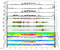
The MMS HPCA measures the distribution of hydrogen, helium, and oxygen ions using an electrostatic analyzer. SPEDAS provides command line and GUI access to HPCA data.
For more information on the HPCA instrument, please see the HPCA Data Products Guide:
https://lasp.colorado.edu/mms/sdc/public/datasets/hpca/ (10160.13 MMS HPCA SCI ALG UM 20160310)
For basic command line access see:
HPCA moments
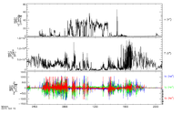
To load and plot HPCA moments for MMS1 on March 7, 2016:
<syntaxhighlight lang="idl"> MMS> mms_load_hpca, probes='1', trange=['2015-10-16', '2015-10-17'], datatype='moments'
MMS> tplot, ['mms1_hpca_hplus_number_density', 'mms1_hpca_oplus_scalar_temperature', 'mms1_hpca_heplus_ion_bulk_velocity'] </syntaxhighlight>
HPCA spectrograms
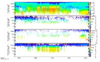
To load and plot HPCA energy spectrograms for MMS1 on March 7, 2016:
<syntaxhighlight lang="idl"> MMS> mms_load_hpca, probes='1', trange=['2015-10-16', '2015-10-17'], datatype='ion'
MMS> mms_hpca_calc_anodes, fov=[0, 360], probe='1'
MMS> tplot, ['mms1_hpca_hplus_flux_elev_0-360', 'mms1_hpca_oplus_flux_elev_0-360', 'mms1_hpca_heplus_flux_elev_0-360', 'mms1_hpca_heplusplus_flux_elev_0-360'] </syntaxhighlight>
SPEDAS derived products
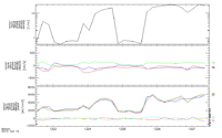
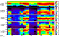
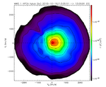
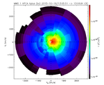
Moments and spectrograms can be calculated from the full 3D distributions using general SPEDAS routines. This allows for various options, such as energy and angle ranges, to be set manually for the calculation.
For example usage see:
Moments
When producing moments all data products are calculated simultaneously for a particular input. Spacecraft potential and magnetic field are specified via supplementary tplot variables.
Spectrograms
Angular spectrograms are calculated in spacecraft and field-aligned coordinates. Phi (azimuth) and theta (elevation) spectra are calculated in spacecraft coordinates. Gyrophase (azimuth) and pitch angle (co-lat) spectra are calculated in field-aligned coordinates. Magnetic field and ephemeris data are specified via supplementary tplot variables. Energy spectrograms are also available.
2D slices
Slices of full 3D particle data can be visualized as smooth contours or by angle/energy bin.
For example usage see:
Visualizing 3D Distribution Functions
- Main article: ISEE_3D
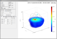
SPEDAS can also be used for visualizing MMS 3D distribution functions from HPCA using the ISEE_3D tool, developed by the Institute for Space-Earth Environmental Research (ISEE), Nagoya University, Japan.
For example usage see:
Example
Load data into tplot <syntaxhighlight lang="idl"> MMS> trange = ['2015-10-20/05:56', '2015-10-20/05:58']
MMS> mms_load_hpca, probe='1', trange=trange, data_rate='srvy', datatype='ion' </syntaxhighlight>
Load the data into standard structures
<syntaxhighlight lang="idl">
MMS> dist = mms_get_dist('mms1_hpca_hplus_phase_space_density', trange=trange)
MMS> data = spd_dist_to_hash(dist) ;convert structures to isee_3d data model </syntaxhighlight>
Load the magnetic field (cyan vector) and velocity (yellow vector) support data
<syntaxhighlight lang="idl">
MMS> mms_load_fgm, probe=1, trange=trange, level='l2'
MMS> mms_load_hpca, probe=1, trange=trange, data_rate='srvy', datatype='moments' </syntaxhighlight>
Once the GUI is opened, select PSD from Units menu
<syntaxhighlight lang="idl">
MMS> isee_3d, data=data, trange=trange, bfield='mms1_fgm_b_gse_srvy_l2_bvec', velocity='mms1_hpca_hplus_ion_bulk_velocity' </syntaxhighlight>
Working with the Data in IDL structures
To get the data out of a tplot variable and into an IDL structure, use get_data:
<syntaxhighlight lang="idl"> MMS> get_data, 'mms1_hpca_azimuth_angles_per_ev_degrees', data=azimuth_angles
MMS> help, azimuth_angles, /structure
Structure <2283cae0>, 5 tags, length=624902264, data length=624902262, refs=1:
X DOUBLE Array[4843]
Y DOUBLE Array[4843, 63, 16, 16]
V1 UINT Array[16]
V2 DOUBLE Array[16]
V3 UINT Array[63]
</syntaxhighlight>
In this example, it's not clear which of the indices of azimuth_angles.Y corresponds to azimuths and which corresponds to anodes. To find out, use print_tinfo:
<syntaxhighlight lang="idl">
MMS> print_tinfo, 'mms1_hpca_azimuth_angles_per_ev_degrees'
Variable: mms1_hpca_azimuth_angles_per_ev_degrees
Structure <2aedf1c0>, 5 tags, length=158709648, data length=158709646, refs=1:
X DOUBLE Array[1230]
Y DOUBLE Array[1230, 63, 16, 16]
V1 UINT Array[16]
V2 DOUBLE Array[16]
V3 UINT Array[63]
Data format: [Epoch_Angles, mms1_hpca_energy_step_number, mms1_hpca_polar_anode_number, mms1_hpca_azimuth_index]
v1: mms1_hpca_azimuth_index
v2: mms1_hpca_polar_anode_number
v3: mms1_hpca_energy_step_number
</syntaxhighlight>