Usage examples: Difference between revisions
(Screenshot of example test_themis_sst added) |
(Caption update) |
||
| (One intermediate revision by the same user not shown) | |||
| Line 8: | Line 8: | ||
This is the script that can be run in IDL: | This is the script that can be run in IDL: | ||
[[File:Test mms1.png|thumb|Screenshot of example test_mms1|upright| | [[File:Test mms1.png|thumb|Screenshot of example test_mms1|upright|400px]] | ||
<code> | <code> | ||
pro test_mms1 | pro test_mms1 | ||
| Line 43: | Line 43: | ||
The scripts in this video are here: | The scripts in this video are here: | ||
[[File:Multiple plot test.png|thumb|Screenshot of example multiple_plot_test| | [[File:Multiple plot test.png|thumb|Screenshot of example multiple_plot_test|400px|right]] | ||
<code> | <code> | ||
| Line 74: | Line 74: | ||
Loading and plotting data from multiple probes: | Loading and plotting data from multiple probes: | ||
[[File:Multiple plot test2.png|thumb|Screenshot of example multiple_plot_test2| | [[File:Multiple plot test2.png|thumb|Screenshot of example multiple_plot_test2|400px|right]] | ||
<code> | <code> | ||
pro multiple_plot_test2 | pro multiple_plot_test2 | ||
| Line 98: | Line 98: | ||
Here is an example script for an SST plot from Themis data: | Here is an example script for an SST plot from Themis data: | ||
[[File:Test themis sst.png|thumb|Screenshot of example Test_themis_sst| | [[File:Test themis sst.png|thumb|Screenshot of example Test_themis_sst|400px]] | ||
<code> | <code> | ||
pro test_themis_sst | pro test_themis_sst | ||
Latest revision as of 19:17, 11 June 2018
SPEDAS contains many introductory scripts that you can run and modify in order to learn using IDL and SPEDAS.
MMS data analysis using SPEDAS: an introduction
This video shows a step-by-step introduction on how to use SPEDAS to make a simple plot:
http://www.youtube.com/watch?v=390FguKn7w4
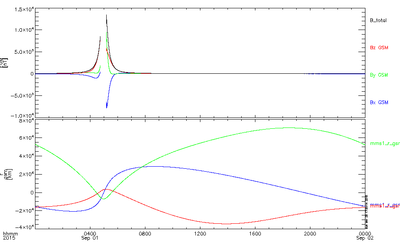
This is the script that can be run in IDL:

pro test_mms1

 mms_init

 ; Select a time range
 trange = ['2015-09-01/21:15', '2015-09-01/21:25']

 ; Select a probe
 probe = 1

 ; Load FGM data
 mms_load_fgm, probe=probe, trange=trange, level='l2'

 ; Load position data
 mms_load_mec, probe=probe, trange=trange, level='l2'

 ; Select quantities to plot
 vars = ['mms1_fgm_b_gsm_srvy_l2', 'mms1_mec_r_gsm']

 ; Plot data
 tplot, vars

end
MMS multi-instrument plots
This video shows how to create multi-panel plots with SPEDAS and how to load data from multiple satellite probes:
http://www.youtube.com/watch?v=yV2NJeiIQsw
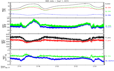
The scripts in this video are here:

pro multiple_plot_test

 mms_init
 trange = ['2015-09-01/21:15', '2015-09-01/21:25']
 probes=['1']
 mms_load_fgm, probes=probes, trange=trange, level='l2'
 mms_load_fpi, probes=probes, trange=trange, level='l2', datatype=['des-moms', 'dis-moms'], data_rate='brst'

 join_vec, 'mms1_des_bulk'+['x', 'y', 'z']+'_dbcs_brst', 'mms1_des_bulk_vel_dbcs'
 join_vec, 'mms1_dis_bulk'+['x', 'y', 'z']+'_dbcs_brst', 'mms1_dis_bulk_vel_dbcs'

 store_data, 'mms1_des_temps_brst', data=['mms1_des_temppara_brst', 'mms1_des_tempperp_brst']
 store_data, 'mms1_dis_temps_brst', data=['mms1_dis_temppara_brst', 'mms1_dis_tempperp_brst']
 store_data, 'mms1_numberdensity_dbcs_brst', data='mms1_d'+['i', 'e']+'s_numberdensity_brst'

 window, 1
 tplot, window=1, title='MMS data - Sept 1, 2015', ['mms1_fgm_b_gsm_srvy_l2', 'mms1_des_bulk_vel_dbcs', 'mms1_des_temps_brst', $
    'mms1_dis_temps_brst', 'mms1_numberdensity_dbcs_brst', 'mms1_des_energyspectr_omni_avg', 'mms1_dis_energyspectr_omni_avg']

 tlimit, trange, window=1

 makepng, "C:\mms\mms_2a", window=1 ; save png file mms_2a.png

end
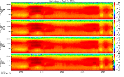
Loading and plotting data from multiple probes:

pro multiple_plot_test2

 mms_init
 trange = ['2015-09-01/21:15', '2015-09-01/21:25']
 probes = ['1','2','3','4']

 mms_load_fpi, probes=probes, trange=trange, level='l2', datatype=['des-moms'], data_rate='brst'

 window, 1
 tplot, window=1, title='MMS data - Sept 1, 2015', ['mms1_des_energyspectr_omni_brst', $
     'mms2_des_energyspectr_omni_brst', 'mms3_des_energyspectr_omni_brst', 'mms4_des_energyspectr_omni_brst']

 tlimit, trange, window=1

 makepng, "C:\mms\mms_2b", window=1  ; save png file mms_2b.png

end
Themis SST plot
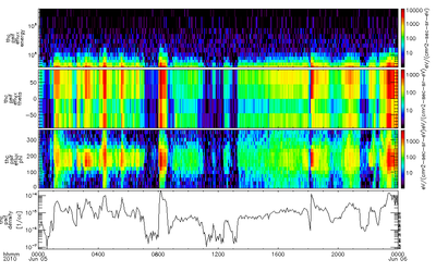
Here is an example script for an SST plot from Themis data:

pro test_themis_sst

 trange = ['2010-06-05','2010-06-06']

 ;set the date and duration (in days)
 timespan,trange

 ;set the spacecraft
 probe = 'c'

 ;set the datatype

 datatype = 'psif' ;(psef for electrons, psib/pseb for burst mode, psir/pser for reduced mode)

 ;loads particle data for data type
 thm_part_load,probe=probe,datatype=datatype

 ;calculate derived products
 thm_part_products,probe=probe,datatype=datatype,trange=trange,outputs =['energy','theta','phi','moments']

 ;view the loaded data names
 tplot_names

 ;plot the energy spectrogram, and angular spectrograms(despun spacecraft coordinates (DSL))
 tplot,['th'+probe+'_psif_eflux_energy','th'+probe+'_psif_eflux_theta','th'+probe+'_psif_eflux_phi','th'+probe+'_psif_density']

end
More examples
The source code of SPEDAS contains many code examples and crib sheets. For each mission included in SPEDAS, there is a directory called "examples" that contains code samples. See the directories:
projects/mms/examples
projects/themis/examples
projects/iugonet/examples
... etc ...