THEMIS Particle Distribution Slices: Difference between revisions
(adding code example, adding images, image moved, clarifying user defined slice alignment) |
(updating eclipse correction section) |
||
| (6 intermediate revisions by the same user not shown) | |||
| Line 1: | Line 1: | ||
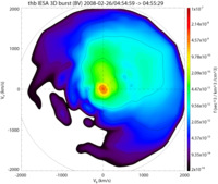
[[File:Themis_slice2d_3d_bv_example.png|200px|thumb|right|THEMIS particle distribution slice using 3D interpolation]] | [[File:Themis_slice2d_3d_bv_example.png|200px|thumb|right|THEMIS particle distribution slice using 3D interpolation]] | ||
THEMIS particle distribution slices plot a two dimensional slices of ESA and/or SST particle data against velocity or energy. Slices are produced after selecting a data type, time window, slice orientation, and z axis units. All samples within the time window are averaged together then the slice is extracted via one of the methods listed below. Slices may be oriented using predefined coordinates or manually. | THEMIS particle distribution slices plot a two dimensional slices of [[THEMIS Electrostatic Analyzer|ESA]] and/or [[THEMIS Solid State Telescope|SST]] particle data against velocity or energy. Slices are produced after selecting a data type, time window, slice orientation, and z axis units. All samples within the time window are averaged together then the slice is extracted via one of the methods listed below. Slices may be oriented using predefined coordinates or manually. | ||
For command line usage see: | For command line usage see: | ||
| Line 21: | Line 21: | ||
==Orientations== | ==Orientations== | ||
All ESA and SST data begins in DSL coordinates. The default orientation of the slice plane is along the x-y plane of the given coordinates. To align the slice plane the following transformations can be applied. | All ESA and SST data begins in DSL coordinates. The default orientation of the slice plane is along the x-y plane of the given coordinates. To align the slice plane the following transformations can be applied. | ||
| Line 60: | Line 61: | ||
'''Note''': If the coordinates and rotation are also set then this transformation will be applied '''after''' those. Therefore, had ''coord="GSM"'' been set in the above statement then the input vectors would be assumed to be in GSM coordinates. Had ''rotation="yz"'' also been set then in the input would be assumed to be in coordinates whose x axis is y<sub>GSM</sub> and whose y axis is z<sub>subGSM</sub>. | '''Note''': If the coordinates and rotation are also set then this transformation will be applied '''after''' those. Therefore, had ''coord="GSM"'' been set in the above statement then the input vectors would be assumed to be in GSM coordinates. Had ''rotation="yz"'' also been set then in the input would be assumed to be in coordinates whose x axis is y<sub>GSM</sub> and whose y axis is z<sub>subGSM</sub>. | ||
==Methods== | ==Interpolation Methods== | ||
====Geometric==== | ====Geometric==== | ||
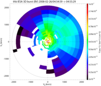
[[File:themis_slice2d_geo_bv_example.png|200px|thumb|right|THEMIS particle distribution slice using the geometric method]] | [[File:themis_slice2d_geo_bv_example.png|200px|thumb|right|THEMIS particle distribution slice using the geometric method]] | ||
| Line 80: | Line 82: | ||
==Units== | ==Units== | ||
Data can be plotted using the following units along the z axis. | Data can be plotted using the following units along the z axis. | ||
{| class="wikitable" style="border: 1px solid LightGray; background-color:#F9F9F9; margin-left:5px;" | {| class="wikitable" style="border: 1px solid LightGray; background-color:#F9F9F9; margin-left:5px;" | ||
| Line 109: | Line 112: | ||
==Smoothing== | ==Smoothing== | ||
[[File:thm_slice_smooth.png|200px|thumb|right|Example of plots with no smoothing vs. default smoothing]] | [[File:thm_slice_smooth.png|200px|thumb|right|Example of plots with no smoothing vs. default smoothing]] | ||
Smoothing is applied using a Gaussian convolution (Gaussian blur). The width of the smoothing window is given in points, therefore higher resolution plots will require wider windows for effective smoothing. Both 3D and 2D interpolation methods default to a smoothing window of 7 points | Smoothing is applied using a Gaussian convolution (Gaussian blur). The width of the smoothing window is given in points, therefore higher resolution plots will require wider windows for effective smoothing. Both 3D and 2D interpolation methods default to a smoothing window of 7 points and a default plot resolution is 150 points. | ||
<div style="border: 1px solid LightGray; background-color:#F9F9F9; padding: 2px 10px; margin-left: 5px; overflow:hidden"> | <div style="border: 1px solid LightGray; background-color:#F9F9F9; padding: 2px 10px; margin-left: 5px; overflow:hidden"> | ||
| Line 117: | Line 121: | ||
==Background Subtraction/Masking== | ==Background Subtraction/Masking== | ||
====ESA background subtraction==== | |||
Background subtraction for ESA data can be applied when loading the input data to ''thm_part_slice2d''. | |||
<div style="border: 1px solid LightGray; background-color:#F9F9F9; padding: 2px 10px; margin-left: 5px; overflow:hidden;"> | |||
SPEDAS> input_data = thm_part_dist_array(probe='a', datatype='peef', trange=[t0,t1], '''/bgnd_remove''') | |||
</div> | |||
For background removal options see [[ESA Background Removal]]. For example usage see: | |||
<div style="border: 1px solid LightGray; background-color:#F9F9F9; padding: 2px 10px; margin-left: 5px; overflow:hidden;"> | |||
/projects/THEMIS/examples/advanced/thm_crib_esa_bgnd_remove.pro | |||
</div> | |||
====SST contamination==== | |||
In most cases, contaminated SST bins should be masked and interpolated over automatically. If the default set of bins is inadequate then a list may be specified instead. | |||
<div style="border: 1px solid LightGray; background-color:#F9F9F9; padding: 2px 10px; margin-left: 5px; overflow:hidden;"> | |||
SPEDAS> thm_part_slice2d, input_data, slice_time=t0, timewin=30, '''sst_sun_bins=[0,8,16,24,32,33,34,40,47,48,49,50,55,56,57]''', part_slice=slice | |||
</div> | |||
For more information see [[SST Contamination Removal]]. | |||
====Count Threshold==== | |||
Two options allow for a minimum count threshold to be set. One options will mask any bins below the specified threshold, while the other will subtract the specified value from the entire distribution. In both cases the operation is applied '''after''' all data from the requested time range has been averaged. | |||
<div style="border: 1px solid LightGray; background-color:#F9F9F9; padding: 2px 10px; margin-left: 5px; overflow:hidden;"> | |||
SPEDAS> thm_part_slice2d, input_data, slice_time=t0, timewin=30, '''count_threshold=1''', part_slice=slice | |||
SPEDAS> thm_part_slice2d, input_data, slice_time=t0, timewin=30, '''subtract_counts=1''', part_slice=slice | |||
</div> | |||
'''Note:''' If the slice window covers a mode change then these operations will be applied '''separately''' to each mode. | |||
==Eclipse Corrections== | ==Eclipse Corrections== | ||
== | Corrections to the spacecraft's spin rate must be loaded for accurate angle determination while the spacecraft is in the Earth's shadow. These corrections are loaded with the particle data and applied automatically when data products are produced. For for information see [[THEMIS Eclipse Corrections]]. | ||
==Resources== | |||
[http://themis.ssl.berkeley.edu/instrument_esa.shtml ESA instrument page] | |||
[http://themis.ssl.berkeley.edu/instrument_sst.shtml SST instrument page] | |||
Latest revision as of 21:37, 28 May 2015

THEMIS particle distribution slices plot a two dimensional slices of ESA and/or SST particle data against velocity or energy. Slices are produced after selecting a data type, time window, slice orientation, and z axis units. All samples within the time window are averaged together then the slice is extracted via one of the methods listed below. Slices may be oriented using predefined coordinates or manually.
For command line usage see:
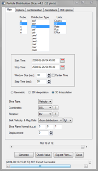
Graphical Interface

The graphical interface may by run with the following call:
This can be used to generate a batches of of plots over a specified time range. Plots will be generated across the entire time range over periods specified by window size and separated by intervals defined by the step time. Once complete, the plots can be browsed using the slider bar at the window's bottom.
Any changes to the Main, Options, and Contamination tabs will require new plots to be generated. The Annotations and Plot Options tabs do not require reprocessing and include Re-Plot buttons to quickly view changes.
Orientations
All ESA and SST data begins in DSL coordinates. The default orientation of the slice plane is along the x-y plane of the given coordinates. To align the slice plane the following transformations can be applied.
Coordinates
A new coordinate system can be used instead of DSL, making the default slice along the x-y plane of those coordinates.
- DSL - The z axis is the spacecraft's spin axis, x is in the direction of the spacecraft-sun vector, y completes the system
- GSM - The x axis is the earth-sun vector, x-z plane contains dipole axis, y axis points towards dusk
- GSE - The x axis is the earth-sun vector, z axis is points towards ecliptic pole, y axis points towards dusk
- xgse - The x axis is the projection of the GSE x-axis
- ygsm - The y axis is the projection of the GSM y-axis
- zdsl - The y axis is the projection of the DSL z-axis
- RGeo - The x is the projection of radial spacecraft position vector (GEI)
- mRGeo - The x axis is the projection of the negative radial spacecraft position vector (GEI)
- phiGeo - The y axis is the projection of the azimuthal spacecraft position vector (GEI), positive eastward
- mphiGeo - The y axis is the projection of the azimuthal spacecraft position vector (GEI), positive westward
- phiSM - The y axis is the projection of the azimuthal spacecraft position vector in Solar Magnetic coords
- mphiSM - The y axis is the projection of the negative azimuthal spacecraft position vector in Solar Magnetic coords
Rotation
The rotation specifies the slice plane's orientation. Some rotations are invariant of the coordinate system (BV, BE, perp) while the rest depend on the starting coordinates.
- BV - The x axis is parallel to B field; the bulk velocity defines the x-y plane
- BE - The x axis is parallel to B field; the B x V(bulk) vector defines the x-y plane
- xy - (default) The x axis is along the coordinate's x axis and y is along the coordinate's y axis
- xz - The x axis is along the coordinate's x axis and y is along the coordinate's z axis
- yz - The x axis is along the coordinate's y axis and y is along the coordinate's z axis
- xvel - The x axis is along the coordinate's x axis; the x-y plane is defined by the bulk velocity
- perp - The x axis is the bulk velocity projected onto the plane normal to the B field; y is B x V(bulk)
- perp_xy - The coordinate's x & y axes are projected onto the plane normal to the B field
- perp_xz - The coordinate's x & z axes are projected onto the plane normal to the B field
- perp_yz - The coordinate's y & z axes are projected onto the plane normal to the B field
User Defined
If another orientation is needed the slice plane can be defined manually. On the command line this is done by setting the slice_norm and (optional) slice_x keyword(s); the former defines the slice plane while the latter's projection defines the slice plane's x axis.
Note: If the coordinates and rotation are also set then this transformation will be applied after those. Therefore, had coord="GSM" been set in the above statement then the input vectors would be assumed to be in GSM coordinates. Had rotation="yz" also been set then in the input would be assumed to be in coordinates whose x axis is yGSM and whose y axis is zsubGSM.
Interpolation Methods
Geometric

The geometric method is effectively a nearest neighbor interpolation. Each data point, or bin, represents a range of possible look directions and energies. Therefore, rather than a standard nearest neighbor algorithm, each point on the plot is given the value of the bin it intersects. At high plot resolutions this allows the boundaries of each bin to be viewed. At low resolutions smaller bins may not be represented. It is recommended to only use this method with the default resolution (500 points).
2D Interpolation
This method projects then linearly interpolates a subset of the distribution onto a regular 2D grid. The set of data used for the interpolation can be chosen by angle from the slice plane or by distance from the slice plane along the plane's normal (km/s if using velocity, eV if using energy). Data that falls within the specified range is be projected onto the slice plane then interpolated. The default selection criteria is ±20° from the slice plane.
3D Interpolation
The entire distribution is linearly interpolated onto a regular 3D grid and a slice is extracted from the volume. The requested plot's resolution also defines the resolution of the interpolated grid (e.g. for the default resolution of 150 the volume will be 150x150x150 points). This method is recommended over 2D interpolation if a true thin slice is required.
Units
Data can be plotted using the following units along the z axis.
| Counts | "counts" | # |
| Rate | "rate" | # / sec |
| Energy Flux | "eflux" | eV / (sec * cm^2 * ster * eV) |
| Flux | "flux" | # / (sec * cm^2 * ster * eV) |
| Distribution Funtion (default) | "df" | f (sec^3 / km^3 /cm^3) |
Smoothing

Smoothing is applied using a Gaussian convolution (Gaussian blur). The width of the smoothing window is given in points, therefore higher resolution plots will require wider windows for effective smoothing. Both 3D and 2D interpolation methods default to a smoothing window of 7 points and a default plot resolution is 150 points.
Background Subtraction/Masking
ESA background subtraction
Background subtraction for ESA data can be applied when loading the input data to thm_part_slice2d.
For background removal options see ESA Background Removal. For example usage see:
SST contamination
In most cases, contaminated SST bins should be masked and interpolated over automatically. If the default set of bins is inadequate then a list may be specified instead.
For more information see SST Contamination Removal.
Count Threshold
Two options allow for a minimum count threshold to be set. One options will mask any bins below the specified threshold, while the other will subtract the specified value from the entire distribution. In both cases the operation is applied after all data from the requested time range has been averaged.
Note: If the slice window covers a mode change then these operations will be applied separately to each mode.
Eclipse Corrections
Corrections to the spacecraft's spin rate must be loaded for accurate angle determination while the spacecraft is in the Earth's shadow. These corrections are loaded with the particle data and applied automatically when data products are produced. For for information see THEMIS Eclipse Corrections.