Analysis Menu - SPEDAS GUI: Difference between revisions
(Initial page from user's guide) |
No edit summary |
||
| (3 intermediate revisions by 2 users not shown) | |||
| Line 1: | Line 1: | ||
[[File:Analysis_menu.png|right | [[File:Analysis_menu.png|right|SPEDAS Analysis Menu]] | ||
The Analysis pull down menu contains selections that allow you to perform various functions on data. The figure on the right shows the Analysis Menu options. | The Analysis pull down menu contains selections that allow you to perform various functions on data. The figure on the right shows the Analysis Menu options. | ||
| Line 69: | Line 69: | ||
=== Power Spectrum === | === Power Spectrum === | ||
[[File:Dproc_power_spectra.png|right|200px|thumb]] | |||
When the Power Spectra button is clicked a new window will be opened containing power spectral parameters that the user can manipulate. The user can choose between dynamic or time power spectra, and select window size and shift, time range and how the data is to be binned. The data is split into components, and a power spectrum is obtained from each component. Appended to the original variable names are "_dpwrspc " or "_tpwrspc” depending on the type of power spectra the user selected, or a suffix can be selected. Note that this is designed for data that are either electric or magnetic field data type. Applying this to other data (e.g., spectrograms) will cause non-intuitive results. | When the Power Spectra button is clicked a new window will be opened containing power spectral parameters that the user can manipulate. The user can choose between dynamic or time power spectra, and select window size and shift, time range and how the data is to be binned. The data is split into components, and a power spectrum is obtained from each component. Appended to the original variable names are "_dpwrspc " or "_tpwrspc” depending on the type of power spectra the user selected, or a suffix can be selected. Note that this is designed for data that are either electric or magnetic field data type. Applying this to other data (e.g., spectrograms) will cause non-intuitive results. | ||
| Line 94: | Line 95: | ||
== Magnetic Field Models == | == Magnetic Field Models == | ||
The SPEDAS GUI can be used to generate and trace geomagnetic field models using the IDL Geopack library. The models currently available from the GUI include IGRF as well as the Tsyganenko 89, 96, 01 and | The SPEDAS GUI can be used to generate and trace geomagnetic field models using the IDL Geopack library. The models currently available from the GUI include IGRF as well as the Tsyganenko 89, 96, 01, 04 and 07 models. To learn more, see [[Magnetic_Field_Models_in_the_SPEDAS_GUI|Magnetic Field Models in the GUI]]. | ||
Latest revision as of 22:59, 15 November 2018
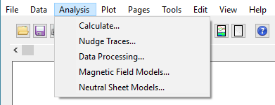
The Analysis pull down menu contains selections that allow you to perform various functions on data. The figure on the right shows the Analysis Menu options.
Calculate
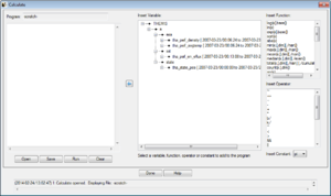
The Calculate Window allows you to access a built in language that will perform simple vector operations on GUI data. The Syntax of the language itself is described in Section 2.5.8 of this manual. Commands for the language can be typed into the text box on the left. Each line will be treated as a separate line. If you want to insert a particular data quantity, just select the quantity from the menu at the right and the quantity will be added to the program text box. You can also insert variables that store the values of numerical constants by selecting them from the drop list in the lower right corner of the window. On the far right side of the window, are drop lists containing common ideal functions and operators. By clicking on an item in the drop list, the function or operator will be inserted into the text box at the last position of the cursor.
Rather than typing your commands in the GUI you can also type a GUI program in a plain text file and load it into the GUI by selecting the 'Open' button at the bottom. If you want to save the program that you currently have in the text box, select the 'Save' button at the bottom of the window.
When you are ready to run the program, select the 'Run' button at the bottom and the Calculate program will be executed. Any quantities that are created will be automatically loaded into the GUI, but if they are much different from the quantities that they came from you may want to double check their meta-data in the manage data menu.
To exit this window, click on the 'X' in the upper right hand corner of the window or the 'OK' button at the bottom of the window. The Calculate window is shown in the figure on the right.
Nudge Traces
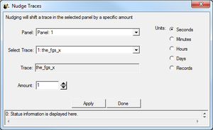
The Nudge Traces option allows the user to “nudge” a trace on a line plot. “Nudging” simply shifts the given trace by a specified amount of time. To activate, select “Nudge Traces” from the “Analysis” pull-down menu on the Main GUI. Note that you need to have created a page and panel and plotted some data before anything will happen when you make this selection. If there has been data plotted, then a window will pop up, allowing you to select the panel, and trace that will be nudged. An example of this window is shown below. There are two drop-down menus that allow you to select the panel and trace that will be nudged. For the current selection, panel 1 is selected, and the trace “tha_state_pos_x” is selected. The units (time units or records) are selected on the right side of the panel; in the example the shift will be given in hours. The number of hours (or minutes, or seconds, etc…) can be selected in the window below the trace selection window. Note that you can type a value into this window as well as use the arrows on the side to scroll values.
When the “Apply” button is clicked, the trace is shifted. This is accomplished by creation of a new variable. The amount of the shift is recorded in the variable name to avoid confusion, to allow for easy recovery of the original values, and to allow a nudged variable to be plotted along with the original. In this example, the new variable name is “tha_state_pos_x_3_hr” and is shown on the panel where the nudged trace is plotted.
Warning: Note that traces are shifted one at a time. If you are attempting to nudge a spectrogram (e.g, THEMIS ESA or SST flux spectrograms, or ASK All Sky Keograms) then you may get unpredictable results when the plot shows up.
Data Processing
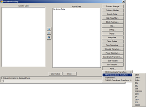
When you click on “Data Processing...” on the Analysis pull-down menu on the Main GUI, a window pops up that allows you certain data processing tasks.
This window is shown below. On the left side is a window that shows the data that has been loaded. You can click on each variable in this window, and set it to “active” by clicking on the right arrow button in between windows. This process works both ways; you can set data to “inactive” by clicking on it in the right-hand window and clicking the left arrow button in the middle. You also have the option to clear the active data by clicking the “Clear Active” button. Data processing tasks are only possible when there is “active” data.
In this window, the “active” data set is “tha_fgh”. Any data processing task will affect these data only. Note that it is not possible to select individual traces for data processing; the full variable is processed.
A data processing task will change the active data set to be the data that has been just been created, so once a task is finished this variable will show up in the right-hand window, and also it will be added to the loaded data tree on the left. Clicking the “Done” button closes the window.
Subtract Average
For each active data set, the average value is subtracted, new variables are created, the new names have the syntax: new_var = old_var+"-d", and the new variables become the active data sets.
Subtract Median
For each active data set, the median value is subtracted, new variables are created, the new names have the syntax: new_var = old_var+"-m", and the new variables become the active data sets.
Smooth Data
This process performs boxcar smoothing of the data. A widget will pop up providing options for this operation, allowing the user to select the resolution of the smoothing window; the default is 61 seconds. You can also determine whether data is smoothed forward from each point, backward from each point, or centered on each point in the data (default). The smoothing operation supports automatic interpolation to a specific cadence. You can also turn on and off check boxes determining whether time interpolation is done, whether true time integration is performed, and whether to smooth NaNs. Finally, you can control the suffix on the output. These options are described in more detail in the header for the SPEDAS routine "smooth_in_time.pro" Select "OK" to process data. "Cancel" or "X" will close the window without processing.
High Pass Filter
Click this button to apply a high-pass filter to the data. The options window that pops up allows you to control the width of the averaging window used to calculate the low pass(which is subtracted from the data to generate the high pass). You can also automatically interpolate to a specific cadence and control the suffix of the output.
Block Average
Click this button to average that data over time. The options window that pops up allows control of the width of each block over which the average is performed. The average can also be limited to a subset of the time range of the data quantities being processed. Finally, you can control the suffix of the output.
Clip
Clips data of the independent variable(y/z axis) in a group to the selected interval. The options window that pops up allows control over the minimum and the maximum for the clipping. You can also control whether points adjacent to the out of range points are also removed. "Insert Flag" allows a particular value to replace clipped values. Finally, "Insert NaNs" allows NaNs to be inserted in place of clipped values. You can also control the suffix appended to the output quantities.
Deflag
Interpolates or repeats the most recent valid data value over gaps in the data (gaps are denoted by NaNs, and can be created by the clipping process; a “deflag” often happens after NaN values are inserted by a “clip” operation). A window pops up to control the parameters for the deflag routine. You can select the method "Repeat Last Value" which will fill flagged regions with the value on the boundary of the region, or "Interpolate" which will interpolate between the values at the boundaries of flagged regions. "Set Flag" allows you to specify the value used as the flag, otherwise NaN is assumed. "Set Maximum Gap" determines the maximum size for a flagged region to be deflagged. You can also control the suffix appended to the resulting quantities.
Degap
The degap procedure locates gaps in data, and fills them in with 'NaN' values, so that the plotting process displays the data gaps correctly (Otherwise it simply draws a line across the gap). It figures out where to add data points by checking which time differences are greater than or equal to an input time interval, plus a margin, and inserts equally spaced 'NaN' data points at time intervals with spacing determined by the size of the data gap divided by the number of points that fit with minimum cumulative error. "Set Flag" allows a value other than NaN to be specified as a flag, and "Set Maximum Gap" allows the maximum gap size to be flagged to be set. You can also control the suffix appended to the resulting quantities.
Clean Spikes
This process removes large single point spikes from messy data. Spikes are identified by removing any regions above a threshold that are larger than a smoothed signal subtracted from the signal. The available settings allow control over how big the difference over the smoothed curve needs to be, and how large a subset of the curve will be included in the smoothing. You can also control the suffix appended to the resulting quantities.
Time Derivative
This process takes the time derivative of the active data sets. The available options allow the data to be smoothed before the derivative is calculated, thereby removing very high frequency components in the derivative. You can also control the suffix appended to the resulting quantities.
Wavelet Transform
The data is split into components, and a basic wavelet transform is performed on each component, with "_wv" appended to the old variable names. (Note that this is designed for data that are either electric or magnetic field data type. Applying this to other data (e.g., spectrograms) will cause non-intuitive results.)
Since this process can be very memory-intensive, the user is first asked to specify a time range. A window allows the user to input start and end times.
Note the values shown here are rough estimates of the available memory and estimated memory usage. If they are close, then it is advisable to click the “NO” button. The process will continue if the “YES” button is pushed. Typical machines have 1 to 2 G-bytes of memory as of this writing (Feb-2009), but if there has been data loaded the available memory may be less. For Window PCs IDL may be limited to 2 GB or less.
Power Spectrum
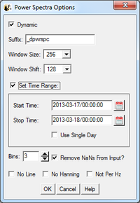
When the Power Spectra button is clicked a new window will be opened containing power spectral parameters that the user can manipulate. The user can choose between dynamic or time power spectra, and select window size and shift, time range and how the data is to be binned. The data is split into components, and a power spectrum is obtained from each component. Appended to the original variable names are "_dpwrspc " or "_tpwrspc” depending on the type of power spectra the user selected, or a suffix can be selected. Note that this is designed for data that are either electric or magnetic field data type. Applying this to other data (e.g., spectrograms) will cause non-intuitive results.
Coordinate Transformation
When the "Coordinate Transform" button is clicked, a dropdown menu appears with different choices for coordinate transforms. Each possible output coordinate system has a button. The possibilities are:
- Despun Spacecraft Coordinates (DSL)
- Spinning Spacecraft Coordinates (SSL)
- Spacecraft Probe Coordinates (SPG)
- Geocentric Solar Magnetospheric (GSM)
- Aberrated Geocentric Solar Magnetospheric (aGSM)
- Geocentric Solar Ecliptic (GSE)
- Geocentric Earth Inertial (GEI)
- Solar Magnetic (SM)
- Selenographic (SEL)
- Selenocentric Solar Ecliptic (SSE)
Only the active data sets are transformed. The input coordinate systems for the active data sets are automatically obtained. Data with "Unknown" coordinates and ground-based data will not be transformed. Note that state data for the appropriate THEMIS probe is necessary for the coordinate transform to occur. If it is not present, then a pop-up will alert the user, and give the option to load the state data.
Click on the "Transform" button to perform the transformation. Warnings and error messages will appear in the text window at the bottom, and also in the progress window on the main widget. Click on the "Close" button to dismiss the popup.
Interpolate
Selecting the interpolate button opens a window containing interpolation options. This function uses the standard IDL interpolate routines. Besides manipulating the interpolation parameters the user can also limit the time range and specify the suffix for the new variable name. Clicking the OK button run the interpolate function on any variables that are in the Active Data area on the Data Processing window.
Magnetic Field Models
The SPEDAS GUI can be used to generate and trace geomagnetic field models using the IDL Geopack library. The models currently available from the GUI include IGRF as well as the Tsyganenko 89, 96, 01, 04 and 07 models. To learn more, see Magnetic Field Models in the GUI.