SPEDAS Developer's Guide: Difference between revisions
No edit summary |
|||
| (29 intermediate revisions by 2 users not shown) | |||
| Line 1: | Line 1: | ||
== Command Line == | == Command Line == | ||
=== Load Data === | |||
Central to all command-line plug-ins in SPEDAS is a routine (typcailly yyy_load_xyz, where YYY is the mission and XYZ is the instrument) or set of routines that grab remote data files from an HTTP/FTP server and loads those data into tplot variables. The simplest way to get started is to host your data on a [https://github.com/hapi-server HAPI server], and implement a yyy_load_xyz routine that loads the XYZ data from your HAPI server using hapi_load_data; the following is a simple example that loads Voyager LECP data: | |||
<syntaxhighlight lang="idl"> | |||
;+ | |||
; NAME: | |||
; voy_load_lecp | |||
; | |||
; PURPOSE: | |||
; Loads Voyager LECP flux data into tplot variables | |||
; | |||
; KEYWORDS: | |||
; PROBE = S/C number to load (default: 1) | |||
; TRANGE = Time range of interest (2 element array), if | |||
; this is not set, the default is to prompt the user. Note | |||
; that if the input time range is not a full day, a full | |||
; days data is loaded | |||
; | |||
; EXAMPLE: | |||
; voy_load_lecp, trange=['1977-09-10', '1977-09-20'], probe=2 | |||
; | |||
;- | |||
pro voy_load_lecp, probe=probe, trange=trange, tplotnames=tplotnames, suffix=suffix | |||
; default to probe 1, and convert to a string if the user does supply the probe via a keyword | |||
if undefined(probe) then probe = '1' else probe = strcompress(string(probe), /remove_all) | |||
; simply load the LECP data from the example server | |||
hapi_load_data, prefix='voy'+probe+'_', $ | |||
trange=trange, $ | |||
suffix=suffix, $ | |||
dataset='spase://VEPO/NumericalData/Voyager'+probe+'/LECP/Flux.Proton.PT1H', $ | |||
server='http://datashop.elasticbeanstalk.com/hapi', $ | |||
tplotnames=tplotnames | |||
end | |||
</syntaxhighlight> | |||
For more information on loading data from HAPI servers, see: [[Heliophysics_Application_Programmer’s_Interface]]. | |||
If your data files are in CDF format, you can download them using spd_download, then load them into tplot variables using cdf2tplot. An example of loading CDF data files can be found below: | |||
<syntaxhighlight lang="idl"> | |||
;+ | |||
; NAME: | |||
; yyy_load_xyz | |||
; | |||
; PURPOSE: | |||
; Loads data from the XYZ instrument onboard the YYY mission into tplot variables | |||
; | |||
; KEYWORDS: | |||
; PROBE = S/C ID to load | |||
; TRANGE = Time range of interest (2 element array), if | |||
; this is not set, the default is to prompt the user. Note | |||
; that if the input time range is not a full day, a full | |||
; days data is loaded | |||
; | |||
; DATATYPE = instrument datatype (allows you to set multiple types of data for | |||
; the instrument) | |||
; | |||
; EXAMPLE: | |||
; yyy_load_xyz, trange=['1977-09-10', '1977-09-20'], probe='2' | |||
; | |||
; NOTES: | |||
; this routine uses MGF data from Geotail hosted at SPDF as an example | |||
; | |||
;- | |||
pro yyy_load_xyz, probe=probe, trange=trange, datatype=datatype, no_color_setup=no_color_setup | |||
; initialize the system variable for this mission | |||
yyy_init, no_color_setup=no_color_setup | |||
; if the user provided a time range via the trange keyword, convert it to doubles | |||
; otherwise, prompt the user for their time range | |||
if (keyword_set(trange) && n_elements(trange) eq 2) $ | |||
then tr = timerange(trange) $ | |||
else tr = timerange() | |||
; set the top level directory for the remote server; this example shows the | |||
; MGF Geotail data at SPDF (so in this example, YYY = Geotail, XYZ = MGF | |||
if not keyword_set(remote_data_dir) then remote_data_dir = 'https://spdf.sci.gsfc.nasa.gov/pub/data/geotail/mgf/' | |||
; set a default datatype if the user did not specify one via the datatype keyword | |||
if undefined(datatype) then datatype = 'edb3sec_mgf' | |||
; next, we need to create an array of paths to the remote filenames; these paths | |||
; start at the remote_data_dir and go all the way to the file extension (i.e., .cdf); | |||
; note that wildcards ('*' and '?') are allowed and encouraged when you do not know part | |||
; of the CDF filename (e.g., the version numbers), and date/times are represented as: | |||
; YYYY = year | |||
; MM = month | |||
; DD = day | |||
; hh = hour | |||
; mm = minute | |||
; ss = second | |||
for datatype_idx = 0, n_elements(datatype)-1 do begin | |||
case strlowcase(datatype[datatype_idx]) of | |||
'eda3sec_mgf': begin | |||
append_array, pathformat, 'eda3sec_mgf/YYYY/ge_eda3sec_mgf_YYYYMMDD_v??.cdf' | |||
end | |||
'edb3sec_mgf': begin | |||
append_array, pathformat, 'edb3sec_mgf/YYYY/ge_edb3sec_mgf_YYYYMMDD_v??.cdf' | |||
end | |||
'mgf_k0': begin | |||
append_array, pathformat, 'mgf_k0/YYYY/ge_k0_mgf_YYYYMMDD_v??.cdf' | |||
end | |||
endcase | |||
endfor | |||
; now we loop over the paths, convert the times using the requesed time range, download | |||
; the data files and load the files into tplot variables | |||
for path_idx = 0, n_elements(pathformat)-1 do begin | |||
; use the file_dailynames routine to convert the time formats in the paths using | |||
; the users requested time range | |||
relpathnames = file_dailynames(file_format=pathformat[path_idx], trange=tr, /unique, resolution=24l*3600) | |||
; use spd_download to download the data to the local data directory | |||
files = spd_download(remote_file=relpathnames, remote_path=remote_data_dir, local_path = local_data_dir, ssl_verify_peer=0, ssl_verify_host=0) | |||
; finally, load the CDF files into tplot variables using cdf2tplot | |||
cdf2tplot, files, /all | |||
endfor | |||
end | |||
</syntaxhighlight> | |||
For reference, the data model for tplot variables can be found at: | |||
http://spedas.org/wiki/index.php?title=Data_model | http://spedas.org/wiki/index.php?title=Data_model | ||
=== Configuration Settings === | |||
The main routine for controlling command-line configuration settings for mission YYY (stored in a system variable called !yyy) is called yyy_init; below is an example yyy_init file. | |||
<syntaxhighlight lang="idl"> | |||
;+ | |||
; NAME: | |||
; yyy_init | |||
; | |||
; PURPOSE: | |||
; Initializes system variables for yyy data. Can be called from idl_startup to set | |||
; custom locations. | |||
;- | |||
pro yyy_init, reset=reset, local_data_dir=local_data_dir, remote_data_dir=remote_data_dir, no_color_setup=no_color_setup | |||
defsysv,'!yyy',exists=exists | |||
if not keyword_set(exists) then begin | |||
defsysv,'!yyy', file_retrieve(/structure_format) | |||
endif | |||
if keyword_set(reset) then !yyy.init=0 | |||
if !yyy.init ne 0 then return | |||
!yyy = file_retrieve(/structure_format) | |||
;Read saved values from file | |||
ftest = yyy_read_config() | |||
If(size(ftest, /type) Eq 8) && ~keyword_set(reset) Then Begin | |||
!yyy.local_data_dir = ftest.local_data_dir | |||
!yyy.remote_data_dir = ftest.remote_data_dir | |||
!yyy.no_download = ftest.no_download | |||
!yyy.no_update = ftest.no_update | |||
!yyy.downloadonly = ftest.downloadonly | |||
!yyy.verbose = ftest.verbose | |||
Endif else begin; use defaults | |||
if keyword_set(reset) then begin | |||
print,'Resetting yyy to default configuration' | |||
endif else begin | |||
print,'No yyy config found...creating default configuration' | |||
endelse | |||
!yyy.local_data_dir = spd_default_local_data_dir() | |||
!yyy.remote_data_dir = '' | |||
endelse | |||
if file_test(!yyy.local_data_dir+'yyy/.master') then begin ; Local directory IS the master directory | |||
!yyy.no_server = 1 | |||
endif | |||
!yyy.init = 1 | |||
printdat,/values,!yyy,varname='!yyy | |||
end | |||
</syntaxhighlight> | |||
=== Part Get Spec (PGS) === | |||
To learn about developing tools that work with particle data, i.e., PGS plug-ins, see: [http://spedas.org/presentations/pgs_development_v1.1.pdf] | |||
== Graphical User Interface (GUI) == | == Graphical User Interface (GUI) == | ||
GUI plug-ins are described by a simple text file located in the folder: spedas_gui/plugins/. Each mission | GUI plug-ins are described by a simple text file located in the folder: spedas_gui/plugins/. Each mission has its own text file describing the various components of the plugin. | ||
Several types of GUI plug-in components are available, including: | Several types of GUI plug-in components are available, including: | ||
* Load Data | * Load Data (load_data) | ||
* Configuration Settings | * Configuration Settings (config) | ||
* Tools Menu | * Tools Menu (menu) | ||
* Data Processing | * Data Processing (data_processing) | ||
* About | * About (about) | ||
A GUI plug-in consists of one or more of the above components, and can have multiple components of any type (e.g., the THEMIS plug-in in SPEDAS contains 2 load_data components, 13 data_processing components, 2 menu components, 1 about component and 1 config component). The suggested way of creating a component for your mission is to fork the example code found in the spedas_gui/api_examples/ folder and modify it for your own mission. | A GUI plug-in consists of one or more of the above components, and can have multiple components of any type (e.g., the THEMIS plug-in in SPEDAS contains 2 load_data components, 13 data_processing components, 2 menu components, 1 about component and 1 config component). The suggested way of creating a component for your mission is to fork the example code found in the spedas_gui/api_examples/ folder and modify it for your own mission. | ||
The following is an example of the GUI plug-in file for the MMS mission; note that all plug-in files must start with "project: " followed by the mission name. | |||
[[File:Mms_plugin_textfile.png|center|MMS Plug-in]] | |||
=== Load Data === | === Load Data === | ||
Load Data (load_data) components allow you to add a new mission tab to the Load Data window found at the menu: | Load Data (load_data) components allow you to add a new mission tab to the Load Data window found at the menu: Data -> Load Data from Plug-ins... These tabs are essentially wrappers around the command-line load routine used to load data into tplot variables. | ||
An example of adding a new tab can be found at: spedas_gui/api_examples/load_data_tab/ | An example of adding a new tab can be found at: spedas_gui/api_examples/load_data_tab/ | ||
| Line 29: | Line 228: | ||
=== Configuration Settings === | === Configuration Settings === | ||
Config Settings components allow you to add a new mission tab to the Configuration Settings window found at the menu: File -> Configuration Settings...; these tabs allow your users to modify various configuration settings that persist through SPEDAS sessions. For most missions, these are wrappers meant to override settings in your mission system variable (!yyy), usually set in yyy_init. For example, config plug-ins allow your users to change the local data directory | Config Settings components allow you to add a new mission tab to the Configuration Settings window found at the menu: File -> Configuration Settings...; these tabs allow your users to modify various configuration settings that persist through SPEDAS sessions. For most missions, these are wrappers meant to override settings in your mission system variable (!yyy), usually set in yyy_init. For example, config plug-ins allow your users to change the local data directory and whether data are downloaded from a remote site or only loaded from the local cache. | ||
An example of adding a new configuration settings tab can be found at: spedas_gui/api_examples/file_configuration_tab/ | |||
[[File:Mms_config.png|340px|center|MMS Config Settings component]] | [[File:Mms_config.png|340px|center|MMS Config Settings component]] | ||
| Line 35: | Line 236: | ||
=== Tools Menu === | === Tools Menu === | ||
Menu components allow you to add a new item to the 'Tools' menu in the GUI. These are currently used in SPEDAS to generate mission overview plots, but can also be used to act as wrappers around more complex functionality (e.g., generating 2D particle slices). | Menu components allow you to add a new item to the 'Tools' menu in the GUI. These are currently used in SPEDAS to generate mission overview plots, but can also be used to act as wrappers around more complex functionality (e.g., generating 2D particle slices for your mission). | ||
An example of adding a new item to the "Tools" menu can be found at: spedas_gui/api_examples/plugin_menu/ | |||
[[File:Tools.png|340px|center|Tools menu component]] | [[File:Tools.png|340px|center|Tools menu component]] | ||
=== Data Processing === | === Data Processing === | ||
Data Processing components allow you to add a new item to the "More..." menu in the "Data Processing" window, found at Analysis -> Data Processing. Data Processing components allow you to add additional data processing operations to the Data Processing window (e.g., mission specific coordinate transformations). | Data Processing components allow you to add a new item to the "More..." menu in the "Data Processing" window, found at Analysis -> Data Processing. Data Processing components allow you to add additional data processing operations to the Data Processing window (e.g., mission specific coordinate transformations). | ||
An example of adding a new item to the "More..." menu in the data processing panel can be found at: spedas_gui/api_examples/data_processing/ | |||
[[File:Data_processing.png|340px|center|Data Processing component]] | [[File:Data_processing.png|340px|center|Data Processing component]] | ||
=== About === | === About === | ||
About components allow you to add a new item describing your mission to the "About SPEDAS Plugins..." menu found at Help -> About. | About components allow you to add a new item describing your mission to the "About SPEDAS Plugins..." menu found at Help -> About. | ||
[[File:About-plugin.png|340px|center|About plugin component]] | |||
Latest revision as of 19:36, 18 March 2019
Command Line
Load Data
Central to all command-line plug-ins in SPEDAS is a routine (typcailly yyy_load_xyz, where YYY is the mission and XYZ is the instrument) or set of routines that grab remote data files from an HTTP/FTP server and loads those data into tplot variables. The simplest way to get started is to host your data on a HAPI server, and implement a yyy_load_xyz routine that loads the XYZ data from your HAPI server using hapi_load_data; the following is a simple example that loads Voyager LECP data:
<syntaxhighlight lang="idl">
- +
- NAME
- voy_load_lecp
- PURPOSE
- Loads Voyager LECP flux data into tplot variables
- KEYWORDS
- PROBE = S/C number to load (default
- 1)
- TRANGE = Time range of interest (2 element array), if
- this is not set, the default is to prompt the user. Note
- that if the input time range is not a full day, a full
- days data is loaded
- EXAMPLE
- voy_load_lecp, trange=['1977-09-10', '1977-09-20'], probe=2
- -
pro voy_load_lecp, probe=probe, trange=trange, tplotnames=tplotnames, suffix=suffix
 ; default to probe 1, and convert to a string if the user does supply the probe via a keyword
 if undefined(probe) then probe = '1' else probe = strcompress(string(probe), /remove_all)

 ; simply load the LECP data from the example server
 hapi_load_data, prefix='voy'+probe+'_', $
                 trange=trange, $
                 suffix=suffix, $
                 dataset='spase://VEPO/NumericalData/Voyager'+probe+'/LECP/Flux.Proton.PT1H', $
                 server='http://datashop.elasticbeanstalk.com/hapi', $
                 tplotnames=tplotnames
end </syntaxhighlight>
For more information on loading data from HAPI servers, see: Heliophysics_Application_Programmer’s_Interface.
If your data files are in CDF format, you can download them using spd_download, then load them into tplot variables using cdf2tplot. An example of loading CDF data files can be found below:
<syntaxhighlight lang="idl">
- +
- NAME
- yyy_load_xyz
- PURPOSE
- Loads data from the XYZ instrument onboard the YYY mission into tplot variables
- KEYWORDS
- PROBE = S/C ID to load
- TRANGE = Time range of interest (2 element array), if
- this is not set, the default is to prompt the user. Note
- that if the input time range is not a full day, a full
- days data is loaded
- DATATYPE = instrument datatype (allows you to set multiple types of data for
- the instrument)
- EXAMPLE
- yyy_load_xyz, trange=['1977-09-10', '1977-09-20'], probe='2'
- NOTES
- this routine uses MGF data from Geotail hosted at SPDF as an example
- -
pro yyy_load_xyz, probe=probe, trange=trange, datatype=datatype, no_color_setup=no_color_setup
 ; initialize the system variable for this mission
 yyy_init, no_color_setup=no_color_setup

 ; if the user provided a time range via the trange keyword, convert it to doubles
 ; otherwise, prompt the user for their time range
 if (keyword_set(trange) && n_elements(trange) eq 2) $
   then tr = timerange(trange) $
 else tr = timerange()

 ; set the top level directory for the remote server; this example shows the
 ; MGF Geotail data at SPDF (so in this example, YYY = Geotail, XYZ = MGF
 if not keyword_set(remote_data_dir) then remote_data_dir = 'https://spdf.sci.gsfc.nasa.gov/pub/data/geotail/mgf/'
 ; set a default datatype if the user did not specify one via the datatype keyword
 if undefined(datatype) then datatype = 'edb3sec_mgf'
 ; next, we need to create an array of paths to the remote filenames; these paths
 ; start at the remote_data_dir and go all the way to the file extension (i.e., .cdf);
 ; note that wildcards ('*' and '?') are allowed and encouraged when you do not know part
 ; of the CDF filename (e.g., the version numbers), and date/times are represented as:
 ; YYYY = year
 ; MM = month
 ; DD = day
 ; hh = hour
 ; mm = minute
 ; ss = second
 for datatype_idx = 0, n_elements(datatype)-1 do begin
   case strlowcase(datatype[datatype_idx]) of
     'eda3sec_mgf': begin
       append_array, pathformat, 'eda3sec_mgf/YYYY/ge_eda3sec_mgf_YYYYMMDD_v??.cdf'
     end
     'edb3sec_mgf': begin
       append_array, pathformat, 'edb3sec_mgf/YYYY/ge_edb3sec_mgf_YYYYMMDD_v??.cdf'
     end
     'mgf_k0': begin
       append_array, pathformat, 'mgf_k0/YYYY/ge_k0_mgf_YYYYMMDD_v??.cdf'
     end
   endcase
 endfor
 ; now we loop over the paths, convert the times using the requesed time range, download
 ; the data files and load the files into tplot variables
 for path_idx = 0, n_elements(pathformat)-1 do begin
   ; use the file_dailynames routine to convert the time formats in the paths using
   ; the users requested time range
   relpathnames = file_dailynames(file_format=pathformat[path_idx], trange=tr, /unique, resolution=24l*3600)
   ; use spd_download to download the data to the local data directory
   files = spd_download(remote_file=relpathnames, remote_path=remote_data_dir, local_path = local_data_dir, ssl_verify_peer=0, ssl_verify_host=0)

   ; finally, load the CDF files into tplot variables using cdf2tplot
   cdf2tplot, files, /all
 endfor
end </syntaxhighlight>
For reference, the data model for tplot variables can be found at:
http://spedas.org/wiki/index.php?title=Data_model
Configuration Settings
The main routine for controlling command-line configuration settings for mission YYY (stored in a system variable called !yyy) is called yyy_init; below is an example yyy_init file.
<syntaxhighlight lang="idl">
- +
- NAME
- yyy_init
- PURPOSE
- Initializes system variables for yyy data. Can be called from idl_startup to set
- custom locations.
- -
pro yyy_init, reset=reset, local_data_dir=local_data_dir, remote_data_dir=remote_data_dir, no_color_setup=no_color_setup
 defsysv,'!yyy',exists=exists
 if not keyword_set(exists) then begin
    defsysv,'!yyy',  file_retrieve(/structure_format)
 endif

 if keyword_set(reset) then !yyy.init=0

 if !yyy.init ne 0 then return

 !yyy = file_retrieve(/structure_format)

 ;Read saved values from file
 ftest = yyy_read_config()

 If(size(ftest, /type) Eq 8) && ~keyword_set(reset) Then Begin
     !yyy.local_data_dir = ftest.local_data_dir
     !yyy.remote_data_dir = ftest.remote_data_dir
     !yyy.no_download = ftest.no_download
     !yyy.no_update = ftest.no_update
     !yyy.downloadonly = ftest.downloadonly
     !yyy.verbose = ftest.verbose
 Endif else begin; use defaults
     if keyword_set(reset) then begin
       print,'Resetting yyy to default configuration'
     endif else begin
       print,'No yyy config found...creating default configuration'
     endelse
     !yyy.local_data_dir = spd_default_local_data_dir()
     !yyy.remote_data_dir =
 endelse

 if file_test(!yyy.local_data_dir+'yyy/.master') then begin  ; Local directory IS the master directory
     !yyy.no_server = 1
 endif

 !yyy.init = 1

 printdat,/values,!yyy,varname='!yyy
end </syntaxhighlight>
Part Get Spec (PGS)
To learn about developing tools that work with particle data, i.e., PGS plug-ins, see: [1]
Graphical User Interface (GUI)
GUI plug-ins are described by a simple text file located in the folder: spedas_gui/plugins/. Each mission has its own text file describing the various components of the plugin.
Several types of GUI plug-in components are available, including:
- Load Data (load_data)
- Configuration Settings (config)
- Tools Menu (menu)
- Data Processing (data_processing)
- About (about)
A GUI plug-in consists of one or more of the above components, and can have multiple components of any type (e.g., the THEMIS plug-in in SPEDAS contains 2 load_data components, 13 data_processing components, 2 menu components, 1 about component and 1 config component). The suggested way of creating a component for your mission is to fork the example code found in the spedas_gui/api_examples/ folder and modify it for your own mission.
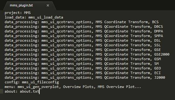
The following is an example of the GUI plug-in file for the MMS mission; note that all plug-in files must start with "project: " followed by the mission name.
Load Data
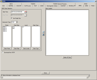
Load Data (load_data) components allow you to add a new mission tab to the Load Data window found at the menu: Data -> Load Data from Plug-ins... These tabs are essentially wrappers around the command-line load routine used to load data into tplot variables.
An example of adding a new tab can be found at: spedas_gui/api_examples/load_data_tab/
Configuration Settings
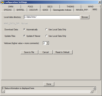
Config Settings components allow you to add a new mission tab to the Configuration Settings window found at the menu: File -> Configuration Settings...; these tabs allow your users to modify various configuration settings that persist through SPEDAS sessions. For most missions, these are wrappers meant to override settings in your mission system variable (!yyy), usually set in yyy_init. For example, config plug-ins allow your users to change the local data directory and whether data are downloaded from a remote site or only loaded from the local cache.
An example of adding a new configuration settings tab can be found at: spedas_gui/api_examples/file_configuration_tab/
Tools Menu
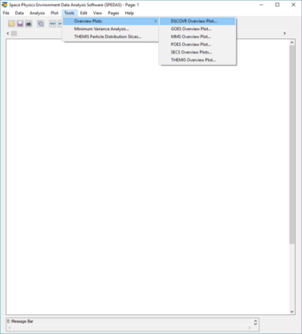
Menu components allow you to add a new item to the 'Tools' menu in the GUI. These are currently used in SPEDAS to generate mission overview plots, but can also be used to act as wrappers around more complex functionality (e.g., generating 2D particle slices for your mission).
An example of adding a new item to the "Tools" menu can be found at: spedas_gui/api_examples/plugin_menu/
Data Processing
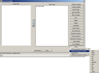
Data Processing components allow you to add a new item to the "More..." menu in the "Data Processing" window, found at Analysis -> Data Processing. Data Processing components allow you to add additional data processing operations to the Data Processing window (e.g., mission specific coordinate transformations).
An example of adding a new item to the "More..." menu in the data processing panel can be found at: spedas_gui/api_examples/data_processing/
About
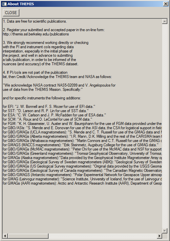
About components allow you to add a new item describing your mission to the "About SPEDAS Plugins..." menu found at Help -> About.
