MMS Fast Plasma Instrument
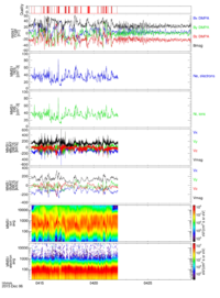
SPEDAS provides command line and GUI access to the MMS FPI data.
Prior to using these data, please read the FPI Release Notes:
https://lasp.colorado.edu/galaxy/display/mms/FPI+Release+Notes
FPI Moments
For more complete examples, see the FPI crib sheets located in the /mms/examples/ folder.
Examples
Electron Moments Data
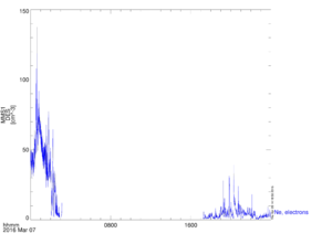
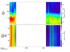
To load and plot the MMS1 FPI electron moments data on March 7, 2016:
MMS> mms_load_fpi, datatype='des-moms', trange=['2016-03-07', '2016-03-08'], probe=1
MMS> tplot, 'mms1_des_numberdensity_dbcs_fast'
MMS> tplot, ['mms1_des_energyspectr_omni_avg', 'mms1_des_pitchangdist_avg']
-
MMS1 FPI electron density on March 7, 2016
-
MMS1 FPI electron energy spectra and pitch angle distribution on March 7, 2016
Ion Moments Data
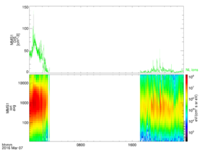
To load and plot the ion density, along with the omni-directional spectra on March 7, 2016:
MMS> mms_load_fpi, datatype='dis-moms', trange=['2016-03-07', '2016-03-08'], probe=1
MMS> tplot, ['mms1_dis_numberdensity_dbcs_fast', 'mms1_dis_energyspectr_omni_avg']
-
MMS1 FPI ion density and energy spectra on March 7, 2016
FPI Distributions
SPEDAS can also be used to load and generate spectra from the FPI distribution functions.
Examples
Electron Distribution Data
To load the FPI electron data:
MMS> mms_load_fpi, probe=1, trange=['2015-10-16/13:02:30', '2015-10-16/13:07:30'], data_rate='brst', datatype='des-dist'
To generate the pitch angle distributions (PADs), we also need spacecraft position and magnetic field data covering the time range:
MMS> mms_load_state, probes=1, trange=['2015-10-16/13:01:30', '2015-10-16/13:08:30']
MMS> mms_load_fgm, probe=1, trange=['2015-10-16/13:01:30', '2015-10-16/13:08:30']
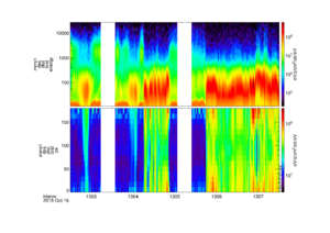
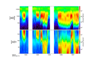
Generate and plot the electron energy spectra and PAD:
MMS> mms_part_products, 'mms1_des_dist_brst', trange=['2015-10-16/13:02:30', '2015-10-16/13:07:30'], mag_name='mms1_fgm_b_dmpa_srvy_l2_bvec', pos_name='mms1_defeph_pos', outputs=['energy','pa']
MMS> tdegap, '*_des_dist_brst_*', /overwrite ; be sure not to interpolate through data gaps
MMS> tplot, ['mms1_des_dist_brst_energy', 'mms1_des_dist_brst_pa']
-
MMS1 FPI electron spectra and PAD on October 16, 2015
Ion Distribution Data
To load the FPI ion data:
MMS> mms_load_fpi, probe=1, trange=['2015-10-16/13:02:30', '2015-10-16/13:07:30'], data_rate='brst', datatype='dis-dist'
To generate the pitch angle distributions (PADs), we also need spacecraft position and magnetic field data covering the time range:
MMS> mms_load_state, probes=1, trange=['2015-10-16/13:01:30', '2015-10-16/13:08:30']
MMS> mms_load_fgm, probe=1, trange=['2015-10-16/13:01:30', '2015-10-16/13:08:30']
Generate and plot the ion energy spectra and PAD:
MMS> mms_part_products, 'mms1_dis_dist_brst', trange=['2015-10-16/13:02:30', '2015-10-16/13:07:30'], mag_name='mms1_fgm_b_dmpa_srvy_l2_bvec', pos_name='mms1_defeph_pos', outputs=['energy','pa']
MMS> tdegap, '*_dis_dist_brst_*', /overwrite ; be sure not to interpolate through data gaps
MMS> tplot, ['mms1_dis_dist_brst_energy', 'mms1_dis_dist_brst_pa']
-
MMS1 FPI ion spectra and PAD on October 16, 2015
FPI 2D Slices
Examples
Basic 2D Slices
Load the FPI ion distribution data:
MMS> mms_load_fpi, data_rate='brst', datatype='dis-dist', probe=1, trange=['2015-10-16/13:06', '2015-10-16/13:07']
Reformat the data for ploting using spd_slice2d:
MMS> dist = mms_get_dist('mms1_dis_dist_brst', trange=['2015-10-16/13:06', '2015-10-16/13:07'])
MMS> slice = spd_slice2d(dist, time='2015-10-16/13:06') ;3D interpolation
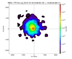
Now plot the slice:
MMS> spd_slice2d_plot, slice
-
MMS1 FPI ion 2D velocity distribution slice at 13:06UT on October 16, 2015
