THEMIS Particle Distribution Slices

File:Themis slice2d 3dbv example.png

THEMIS particle distribution slice

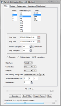
THEMIS particle distribution slices plot a two dimensional slices of ESA and/or SST particle data against velocity or energy. Slices are produced after selecting a data type, time window, slice orientation, and z axis units. All samples within the time window are averaged together then the slice is extracted via one of the methods listed below. Slices may be oriented using predefined coordinates or manually.

For command line usage see:

/projects/THEMIS/examples/basic/thm_crib_part_slice2d.pro

Graphical Interface

Graphical interface for producing distribution slices

The graphical interface may by run with the following call:

SPEDAS> thm_ui_slice2d

This can be used to generate a batches of of plots over a specified time range. Plots will be generated across the entire time range over periods specified by window size and separated by intervals defined by the step time. Once complete, the plots can be browsed using the slider bar at the window's bottom.

Any changes to the Main, Options, and Contamination tabs will require new plots to be generated. The Annotations and Plot Options tabs do not require reprocessing and include Re-Plot buttons to quickly view changes.

Orientations

All ESA and SST data begins in DSL coordinates. The default orientation of the slice plane is along the x-y plane of the given coordinates. To align the slice plane the following transformations can be applied.

A new coordinate system can be used instead of DSL, making the default slice along the x-y plane of those coordinates.

• DSL -
• GSM - The x axis is the earth-sun vector, x-z plane contains dipole axis, y axis points towards dusk
• GSE - The x axis is the earth-sun vector, z axis is points towards ecliptic pole, y axis points towards dusk
• xgse - The x axis is the projection of the GSE x-axis
• ygsm - The y axis is the projection of the GSM y-axis
• zdsl - The y axis is the projection of the DSL z-axis
• RGeo - The x is the projection of radial spacecraft position vector (GEI)
• mRGeo - The x axis is the projection of the negative radial spacecraft position vector (GEI)
• phiGeo - The y axis is the projection of the azimuthal spacecraft position vector (GEI), positive eastward
• mphiGeo - The y axis is the projection of the azimuthal spacecraft position vector (GEI), positive westward
• phiSM - The y axis is the projection of the azimuthal spacecraft position vector in Solar Magnetic coords
• mphiSM - The y axis is the projection of the negative azimuthal spacecraft position vector in Solar Magnetic coords

Rotation

The rotation specifies the slice plane's orientation. Some rotations are invariant of the coordinate system (BV, BE, perp) while the rest depend on the starting coordinates.

• BV - The x axis is parallel to B field; the bulk velocity defines the x-y plane
• BE - The x axis is parallel to B field; the B x V(bulk) vector defines the x-y plane
• xy - (default) The x axis is along the coordinate's x axis and y is along the coordinate's y axis
• xz - The x axis is along the coordinate's x axis and y is along the coordinate's z axis
• yz - The x axis is along the coordinate's y axis and y is along the coordinate's z axis
• xvel - The x axis is along the coordinate's x axis; the x-y plane is defined by the bulk velocity
• perp - The x axis is the bulk velocity projected onto the plane normal to the B field; y is B x V(bulk)
• perp_xy - The coordinate's x & y axes are projected onto the plane normal to the B field
• perp_xz - The coordinate's x & z axes are projected onto the plane normal to the B field
• perp_yz - The coordinate's y & z axes are projected onto the plane normal to the B field

User Defined

If another orientation is needed the slice plane can be defined manually. On the command line this is done by setting the slice_norm and (optional) slice_x keyword(s); the former defines the slice plane while the latter projection define's the slice plane's x axis.

SPEDAS> thm_part_slice2d, data, slice_time=t0, timewin=30, slice_norm=[1,2,3], slice_x=[1,-2,3], part_slice=slice

Note: If the coordinates and rotation are also set then this transformation will be applied after those. Therefore, had coord="GSM" been set in the above statement then the input vectors would be assumed to be in GSM coordinates. Had rotation="yz" also been set then in the input would be assumed to be in GSM coordinates with x, y, and z axes rotated to z, x, and y respectively.

Methods

Geomtric

Each point on the plot is given the value of the bin it instersects. This allows bin boundaries to be drawn at high resolutions.

2D Interpolation

Datapoints within the specified theta or z-axis range are projected onto the slice plane and linearly interpolated onto a regular 2D grid.

3D Interpolation

The entire 3-dimensional distribution is linearly interpolated onto a regular 3D grid and a slice is extracted from the volume. Interpolation may occur across data gaps or areas with recorded zeroes.

Units

Available z axis units:

Counts	#
Rate	# / sec
Energy Flux	eV / (sec * cm^2 * ster * eV)
Flux	# / (sec * cm^2 * ster * eV)
df	f (sec^3 / km^3 /cm^3)