Data Menu - SPEDAS GUI

SPEDAS Data Menu

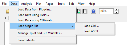
The SPEDAS GUI can be used to load data from a number of missions, including THEMIS, GOES, FAST, WIND, ACE, IUGONET and OMNI. The GUI can also be used to load data from HAPI Web Services and from the SPDF CDAWeb. It can also load local ASCII and CDF files.

Load Data from Plug-ins

The Load Data from Plug-ins option, opens a window that allows the user to select specific data sets to be loaded into memory using SPEDAS plugins.

SPEDAS is a modular application and every supported mission is a different module. Each mission supplies its own Load Data widget which is loaded into the Load Data window as a separate tab. The following image shows the Load Data window with the THEMIS mission data load tab. However, the Load Data window might look different in your setup, depending on which mission modules have been added to SPEDAS.

Load Data Window

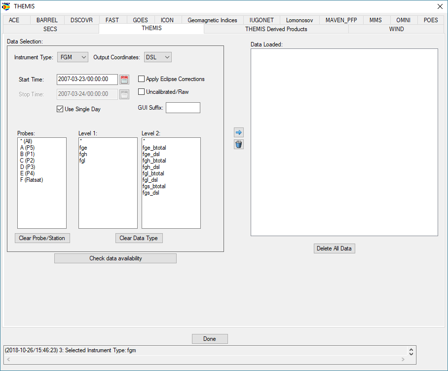
Each mission has its own way of loading data with GUI elements specific to the mission. In general, we have to choose the instrument, a data range and then we have to click the arrow to load the data into SPEDAS.

The left hand side of the window contains the data selection area and the right hand side of the window displays data that has already been loaded.

Data can be removed at any time by making a selection in the data tree and clicking the trash can. The data tree will be updated to reflect the deletion. The user can also use the Clear All button below the data tree to delete all data.

At the bottom of the window is a status bar. Messages regarding the load process, data, and/or status of the window will be displayed here.

When you have loaded all the data you want, click the Done button below the data tree.

Load Data using HAPI

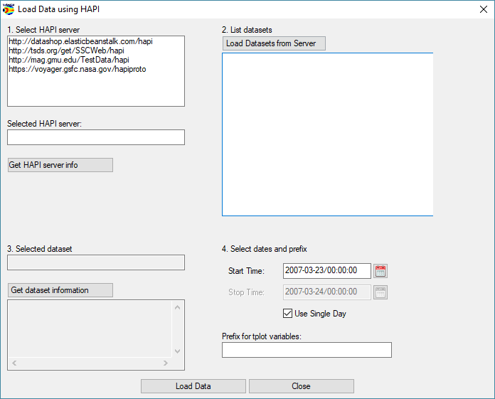
The "Load Data using HAPI" dialog allows the user to load data using a HAPI web service. It opens a new window where the user can select a HAPI server, view the datasets in that HAPI server, and load a particular dataset for a particular time span.

Load Data using HAPI Window

For more information on HAPI, see:

https://cdaweb.sci.gsfc.nasa.gov/registry/hdp/hapi/

Load Data using CDAWlib

The "Load Data using CDAWeb" dialog allows the user to load data from a large number of NASA missions. The CDAWeb graphical download tool was originally developed by NASA. For information on the NASA tools for IDL, see:

https://cdaweb.gsfc.nasa.gov/WebServices/REST/CdasIdlLibrary.html

We have adapted their code to the needs of SPEDAS and the result is an integrated download tool that can receive data from dozens of mission and transform this data to the tplot format used in SPEDAS. Then the data can be plotted or transformed like any other data set. The following figure shows the CDAWeb Data Chooser window.

Load Data using CDAWeb Window

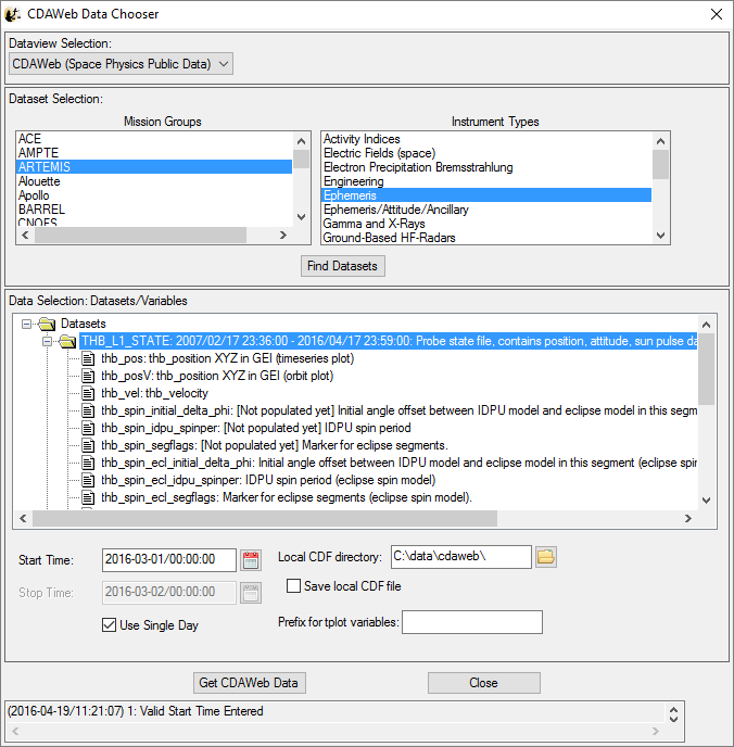
To use the tool, first select the mission name (for example, “ARTEMIS”) and the type of the instruments (for example, “Magnetic Fields (space)”) and then click the button “Find Datasets”. This gives a list of all available data sets and the dates of availability of each data set. Expand the data sets and select one or more data variables (using Ctrl+Click to select multiple variables). We can select the start and end dates and times using the calendar widget. We have to pick dates that are within the availability dates of the particular data set we have selected. It is also important to select a “Local CDF directory” which is writable, because that directory will be used to download files for the CDAWeb data repository, even if we do not retain those files. If we want to keep the downloaded CDF files, then we should check the checkbox “Save local CDF file”. We can also define an optional prefix for the resulting variables, for example “artemis_”. Clicking on the “Get CDAWeb Data” button downloads the requested data set. After the download is complete, we get a message that informs us that the download was successful (or not) and another window which allows us to specify the name of the tplot parameter names. This last window is the same as when we import data from an arbitrary CDF file. After this, the CDAWeb Data Chooser window closes and we can work with the data we have downloaded.

Load Single File

The Load Single File option allows the user to load data from CDF or ASCII files in his local computer.

Manage Tplot and GUI Variables

SPEDAS verify data

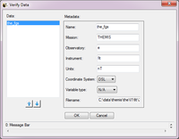
The Manage Tplot and GUI Variables option allows the user to (1) import TPLOT variables into GUI Variables, (2) export GUI Variables into TPLOT Variables, (3) delete GUI variables, and (4) view/edit the meta-data associated with various GUI variables.

To import TPLOT variables you can select one or many (ctrl/shift-click) tplot variables in the left TPLOT Data area, then press the right arrow button to move data into the GUI. The data will then be moved into the GUI and attempt to detect the variable meta-data that includes name, mission, observatory, instrument, units, and coordinate system.

When the right arrow is clicked to import tplot data, the Verify Data Window will be displayed allowing you to verify that this data was correctly detected. Click the OK button if it is or 'Cancel' if you change your mind about importing. After you press 'OK' on the Verify Data panel, the data will be loaded. The figure to the right shows the Verify Data window.

To export GUI variables to TPLOT, select the GUI quantities that you would like to export from the tree at the right and select the left arrow button to export them.

To delete GUI variables, select the GUI quantities that you would like to delete from the tree at the right, then select the trash can button to delete them.

To examine the meta-data (name, mission, observatory, instrument, units, coordinate system, and file name) associated with particular GUI variables. Select the variable to be examined in the tree at the right and select the magnifying glass button to examine the meta-data. A menu like the verify menu will pop-up and you can view or edit the meta-data for the selected quantities.

Save Data As

The "Save Data As" option allows the user to select a set of variables, and save the data as ASCII (with various formatting options) or as a set of files in the UCLA binary "upper flat file" format. Unlike "Save SPEDAS Document" or "Save As…", "Save Data As…" does not attempt to save any GUI objects or plotting parameters.

Click "Data->Save Data As" to bring up the dialog. On Windows XP, it will look something like this, assuming some data has already been loaded:

SPEDAS Save Data As...

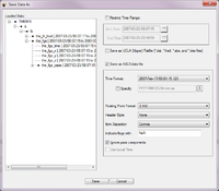
The left hand "Loaded Data" pane is a "tree widget" representing the data variables currently available. In the above screen shot, many of the nodes are fully expanded. Click any box showing "+" to expand that node, or click a box showing "-" to collapse that node.

To the right of the "Loaded Data" pane are some additional controls. If the "Restrict Time Range" box is checked, only the data with timestamps in the given time range will be saved. For now, the start and end times must be typed into the text box in YYYY-MM-DD/HH:MM:SS format.

If the "Save as Flat file" box is checked, the data will be saved in (binary) UCLA flat file format. For further information about this format, please consult the UCLA documentation.

If the "Save as ASCII data file" box is checked, the data will be saved as ASCII, one line per record. If this format is selected, there are additional choices for how the ASCII data is formatted. The "Time Format" drop-down menu brings up a list of different formats for representing timestamps with varying degrees of precision. The "Floating Point Format" drop-down menu specifies the precision and format of floating point quantities that are not internally marked as timestamps.

The "Header Style" drop-down menu offers a few options for including header lines in the ASCII output. If "None" is selected, no header will be produced; for "Field Names Only", a single header line will be included, listing the field names associated with each data column; for "Tecplot", a Tecplot-compatible header will be produced with one line of field names, and another line with a sample count and some other information.

The "Item Separator" drop-down menu allows the user to select whether columns are to be separated by commas, tabs, or spaces. This option also applies to the header, if one is requested.

As an example, if "Header Style" is set to "Field Names Only" and "Item Separator" is set to "Comma", the resulting ASCII file should be readable by Excel or other utilities that understand CSV ("comma separated value") formatted files.

The "Indicate flags with:" text box allows the user to choose what gets printed if an IEEE-754 "NaN", "Inf", or other non-numeric floating point value is encountered during the conversion to ASCII. We suggest keeping the default text "NaN". (The term "flag" is used because in some situations, TDAS inserts NaN values to "flag" missing or invalid data samples.)

"Update document with location of data" is not yet implemented in this release (and perhaps never will be), and should be disregarded for now.

The suggested workflow for this dialog is to first use the tree widget in the "Loaded Data" pane to select some subset of the currently loaded variables, then use the controls on the right hand side to select a file format, an optional time range, and any additional style settings (if ASCII format is selected). Clicking the "Save" button will perform a few checks on the selected data variables, and if the selection is valid, the GUI will pop up a file picker dialog to specify the filename and directory to save.

Caveats:

This dialog does not permit saving arbitrary collections of variables. Owing to the record-oriented structure of these file formats, all selected variables must contain the same number of samples. For UCLA upper flat file format, the only valid data types are 4-byte integers, and 4- and 8-byte floating-point values. THEMIS data represented as bytes or 16-bit integers (for example, ASK) cannot be saved as UCLA upper flat files. These restrictions are enforced at the very end of the workflow, when the user clicks "Save". The first variable name with an incompatible sample count or data type will be mentioned in the error message; try removing that variable from the selection, and repeat the process until a valid ensemble of variables remains.

ASCII files generated from large data sets (e.g. several hours of ASK keogram data) are potentially enormous, and may appear to lock up IDL for a long time while the file is being written. Even modest ASCII data sets may require several minutes to be saved. These operations are somewhat inefficient; due to the need for column-by-column checking, formatting, and output of data fields.