MMS Fast Plasma Instrument: Difference between revisions
(adding syntax highlighting to code snippets) |
|||
| (13 intermediate revisions by the same user not shown) | |||
| Line 15: | Line 15: | ||
=== Electron Moments Data === | === Electron Moments Data === | ||
To load and plot the MMS1 FPI electron moments data on March 7, 2016: | To load and plot the MMS1 FPI electron moments data on March 7, 2016: | ||
< | <syntaxhighlight lang="idl"> | ||
MMS> mms_load_fpi, datatype='des-moms', trange=['2016-03-07', '2016-03-08'], probe=1 | MMS> mms_load_fpi, datatype='des-moms', trange=['2016-03-07', '2016-03-08'], probe=1 | ||
MMS> tplot, 'mms1_des_numberdensity_fast' | MMS> tplot, 'mms1_des_numberdensity_fast' | ||
MMS> tdegap, ['mms1_des_energyspectr_omni_fast', 'mms1_des_pitchangdist_avg'], /overwrite | |||
MMS> tplot, ['mms1_des_energyspectr_omni_fast', 'mms1_des_pitchangdist_avg'] | MMS> tplot, ['mms1_des_energyspectr_omni_fast', 'mms1_des_pitchangdist_avg'] | ||
</ | </syntaxhighlight> | ||
| Line 31: | Line 33: | ||
=== Ion Moments Data === | === Ion Moments Data === | ||
To load and plot the ion density, along with the omni-directional spectra on March 7, 2016: | To load and plot the ion density, along with the omni-directional spectra on March 7, 2016: | ||
< | <syntaxhighlight lang="idl"> | ||
MMS> mms_load_fpi, datatype='dis-moms', trange=['2016-03-07', '2016-03-08'], probe=1 | MMS> mms_load_fpi, datatype='dis-moms', trange=['2016-03-07', '2016-03-08'], probe=1 | ||
MMS> tdegap, ['mms1_dis_numberdensity_fast', 'mms1_dis_energyspectr_omni_fast'], /overwrite | |||
MMS> tplot, ['mms1_dis_numberdensity_fast', 'mms1_dis_energyspectr_omni_fast'] | MMS> tplot, ['mms1_dis_numberdensity_fast', 'mms1_dis_energyspectr_omni_fast'] | ||
</ | </syntaxhighlight> | ||
| Line 43: | Line 47: | ||
= FPI Distributions = | = FPI Distributions = | ||
SPEDAS can also be used to | SPEDAS can also be used to generate secondary data products (energy, gyrophase, PA spectra) from the FPI distribution functions. | ||
== Examples == | == Examples == | ||
| Line 50: | Line 54: | ||
Generate and plot the electron energy spectra and PAD from the FPI distribution functions: | Generate and plot the electron energy spectra and PAD from the FPI distribution functions: | ||
< | <syntaxhighlight lang="idl"> | ||
MMS> mms_part_getspec, instrument='fpi', probe='1', species='e', data_rate='brst', level='l2', outputs=['energy', 'pa'], trange=['2015-10-16/13:02:30', '2015-10-16/13:07:30'] | MMS> mms_part_getspec, instrument='fpi', probe='1', species='e', data_rate='brst', level='l2', outputs=['energy', 'pa'], trange=['2015-10-16/13:02:30', '2015-10-16/13:07:30'] | ||
| Line 57: | Line 61: | ||
MMS> tplot, ['mms1_des_dist_brst_energy', 'mms1_des_dist_brst_pa'] | MMS> tplot, ['mms1_des_dist_brst_energy', 'mms1_des_dist_brst_pa'] | ||
</ | </syntaxhighlight> | ||
<gallery widths=300px heights=250px align="center"> | <gallery widths=300px heights=250px align="center"> | ||
Mms_part_products_fpi_spec.png|MMS1 FPI electron spectra and PAD on October 16, 2015 | Mms_part_products_fpi_spec.png|MMS1 FPI electron spectra and PAD on October 16, 2015 | ||
</gallery> | |||
To generate angle-angle plots from the FPI electron distribution functions at a specific time: | |||
<syntaxhighlight lang="idl"> | |||
MMS> mms_fpi_ang_ang, '2015-10-16/13:07:30', species='e', data_rate='brst' | |||
</syntaxhighlight> | |||
<gallery widths=300px heights=250px align="center"> | |||
Azimuth_vs_zenith_electrons.png| | |||
Azimuth_vs_energy_electrons.png| | |||
Zenith_vs_energy_electrons.png| | |||
Pad_vs_energy_electrons.png| | |||
</gallery> | </gallery> | ||
=== Ion Distribution Data === | === Ion Distribution Data === | ||
Generate and plot the ion energy spectra and PAD: | Generate and plot the ion energy spectra and PAD from the FPI distribution functions: | ||
< | <syntaxhighlight lang="idl"> | ||
MMS> mms_part_getspec, instrument='fpi', probe='1', species='i', data_rate='brst', level='l2', outputs=['energy', 'pa'], trange=['2015-10-16/13:02:30', '2015-10-16/13:07:30'] | MMS> mms_part_getspec, instrument='fpi', probe='1', species='i', data_rate='brst', level='l2', outputs=['energy', 'pa'], trange=['2015-10-16/13:02:30', '2015-10-16/13:07:30'] | ||
| Line 74: | Line 94: | ||
MMS> tplot, ['mms1_dis_dist_brst_energy', 'mms1_dis_dist_brst_pa'] | MMS> tplot, ['mms1_dis_dist_brst_energy', 'mms1_dis_dist_brst_pa'] | ||
</ | </syntaxhighlight> | ||
<gallery widths=300px heights=250px align="center"> | <gallery widths=300px heights=250px align="center"> | ||
Mms_part_products_ion_spec.png|MMS1 FPI ion spectra and PAD on October 16, 2015 | Mms_part_products_ion_spec.png|MMS1 FPI ion spectra and PAD on October 16, 2015 | ||
</gallery> | |||
To generate angle-angle plots from the FPI ion distribution functions at a specific time: | |||
<syntaxhighlight lang="idl"> | |||
MMS> mms_fpi_ang_ang, '2015-10-16/13:07:30', species='i', data_rate='brst' | |||
</syntaxhighlight> | |||
<gallery widths=300px heights=250px align="center"> | |||
Azimuth_vs_zenith_ions.png| | |||
Azimuth_vs_energy_ions.png| | |||
Zenith_vs_energy_ions.png| | |||
Pad_vs_energy_ions.png| | |||
</gallery> | </gallery> | ||
| Line 89: | Line 125: | ||
Load the FPI ion distribution data: | Load the FPI ion distribution data: | ||
< | <syntaxhighlight lang="idl"> | ||
MMS> mms_load_fpi, data_rate='brst', datatype='dis-dist', probe=1, trange=['2015-10-16/13:06', '2015-10-16/13:07'] | MMS> mms_load_fpi, data_rate='brst', datatype='dis-dist', probe=1, trange=['2015-10-16/13:06', '2015-10-16/13:07'] | ||
</ | </syntaxhighlight> | ||
Reformat the data for | Reformat the data for plotting using spd_slice2d: | ||
< | <syntaxhighlight lang="idl"> | ||
MMS> dist = mms_get_dist('mms1_dis_dist_brst', trange=['2015-10-16/13:06', '2015-10-16/13:07']) | MMS> dist = mms_get_dist('mms1_dis_dist_brst', trange=['2015-10-16/13:06', '2015-10-16/13:07']) | ||
| Line 104: | Line 140: | ||
MMS> slice = spd_slice2d(dist, time='2015-10-16/13:06') ;3D interpolation | MMS> slice = spd_slice2d(dist, time='2015-10-16/13:06') ;3D interpolation | ||
</ | </syntaxhighlight> | ||
Now plot the slice: | Now plot the slice: | ||
< | <syntaxhighlight lang="idl"> | ||
MMS> spd_slice2d_plot, slice | MMS> spd_slice2d_plot, slice | ||
</ | </syntaxhighlight> | ||
| Line 125: | Line 161: | ||
Load data into tplot | Load data into tplot | ||
< | <syntaxhighlight lang="idl"> | ||
MMS> mms_load_fpi, probe=1, trange=['2015-10-20/05:56:30', '2015-10-20/05:56:34'], data_rate='brst', datatype='dis-dist' | MMS> mms_load_fpi, probe=1, trange=['2015-10-20/05:56:30', '2015-10-20/05:56:34'], data_rate='brst', datatype='dis-dist' | ||
</ | </syntaxhighlight> | ||
Load the data into standard structures | Load the data into standard structures | ||
< | <syntaxhighlight lang="idl"> | ||
MMS> dist = mms_get_fpi_dist('mms1_dis_dist_brst' , trange=['2015-10-20/05:56:30', '2015-10-20/05:56:34']) | MMS> dist = mms_get_fpi_dist('mms1_dis_dist_brst' , trange=['2015-10-20/05:56:30', '2015-10-20/05:56:34']) | ||
| Line 139: | Line 175: | ||
MMS> data = spd_dist_to_hash(dist) ;convert structures to isee_3d data model | MMS> data = spd_dist_to_hash(dist) ;convert structures to isee_3d data model | ||
</ | </syntaxhighlight> | ||
Load the magnetic field (cyan vector) and velocity (yellow vector) support data | Load the magnetic field (cyan vector) and velocity (yellow vector) support data | ||
< | <syntaxhighlight lang="idl"> | ||
MMS> mms_load_fgm, probe=1, trange=['2015-10-20/05:55:30', '2015-10-20/05:57:34'], level='l2' | MMS> mms_load_fgm, probe=1, trange=['2015-10-20/05:55:30', '2015-10-20/05:57:34'], level='l2' | ||
| Line 149: | Line 185: | ||
MMS> mms_load_fpi, data_rate='brst', datatype='dis-moms', probe=1, trange=['2015-10-20/05:56:30', '2015-10-20/05:56:34'] | MMS> mms_load_fpi, data_rate='brst', datatype='dis-moms', probe=1, trange=['2015-10-20/05:56:30', '2015-10-20/05:56:34'] | ||
</syntaxhighlight> | |||
</ | |||
Once the GUI is opened, select PSD from Units menu | Once the GUI is opened, select PSD from Units menu | ||
< | <syntaxhighlight lang="idl"> | ||
MMS> isee_3d, data=data, trange=['2015-10-20/05:56:30', '2015-10-20/05:56:34'], bfield='mms1_fgm_b_gse_srvy_l2_bvec', velocity=' | MMS> isee_3d, data=data, trange=['2015-10-20/05:56:30', '2015-10-20/05:56:34'], bfield='mms1_fgm_b_gse_srvy_l2_bvec', velocity='mms1_dis_bulkv_dbcs_brst' | ||
</ | </syntaxhighlight> | ||
Latest revision as of 19:13, 29 March 2018

SPEDAS provides command line and GUI access to the MMS FPI data.
Prior to using these data, please read the FPI Release Notes:
https://lasp.colorado.edu/mms/sdc/public/datasets/fpi/ (FPI Release Notes)
FPI Moments
For more complete examples, see the FPI crib sheets located in the /mms/examples/ folder.
Examples
Electron Moments Data
To load and plot the MMS1 FPI electron moments data on March 7, 2016: <syntaxhighlight lang="idl"> MMS> mms_load_fpi, datatype='des-moms', trange=['2016-03-07', '2016-03-08'], probe=1
MMS> tplot, 'mms1_des_numberdensity_fast'
MMS> tdegap, ['mms1_des_energyspectr_omni_fast', 'mms1_des_pitchangdist_avg'], /overwrite
MMS> tplot, ['mms1_des_energyspectr_omni_fast', 'mms1_des_pitchangdist_avg'] </syntaxhighlight>
-
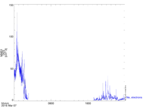
MMS1 FPI electron density on March 7, 2016
-
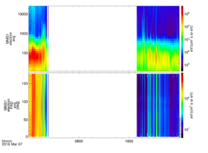
MMS1 FPI electron energy spectra and pitch angle distribution on March 7, 2016


Ion Moments Data
To load and plot the ion density, along with the omni-directional spectra on March 7, 2016: <syntaxhighlight lang="idl"> MMS> mms_load_fpi, datatype='dis-moms', trange=['2016-03-07', '2016-03-08'], probe=1
MMS> tdegap, ['mms1_dis_numberdensity_fast', 'mms1_dis_energyspectr_omni_fast'], /overwrite
MMS> tplot, ['mms1_dis_numberdensity_fast', 'mms1_dis_energyspectr_omni_fast'] </syntaxhighlight>
-
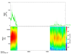
MMS1 FPI ion density and energy spectra on March 7, 2016

FPI Distributions
SPEDAS can also be used to generate secondary data products (energy, gyrophase, PA spectra) from the FPI distribution functions.
Examples
Electron Distribution Data
Generate and plot the electron energy spectra and PAD from the FPI distribution functions:
<syntaxhighlight lang="idl"> MMS> mms_part_getspec, instrument='fpi', probe='1', species='e', data_rate='brst', level='l2', outputs=['energy', 'pa'], trange=['2015-10-16/13:02:30', '2015-10-16/13:07:30']
MMS> tdegap, '*_des_dist_brst_*', /overwrite ; be sure not to interpolate through data gaps
MMS> tplot, ['mms1_des_dist_brst_energy', 'mms1_des_dist_brst_pa']
</syntaxhighlight>
-
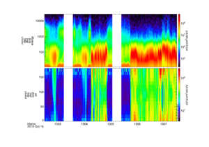
MMS1 FPI electron spectra and PAD on October 16, 2015

To generate angle-angle plots from the FPI electron distribution functions at a specific time:
<syntaxhighlight lang="idl"> MMS> mms_fpi_ang_ang, '2015-10-16/13:07:30', species='e', data_rate='brst'
</syntaxhighlight>


Ion Distribution Data
Generate and plot the ion energy spectra and PAD from the FPI distribution functions:
<syntaxhighlight lang="idl"> MMS> mms_part_getspec, instrument='fpi', probe='1', species='i', data_rate='brst', level='l2', outputs=['energy', 'pa'], trange=['2015-10-16/13:02:30', '2015-10-16/13:07:30']
MMS> tdegap, '*_dis_dist_brst_*', /overwrite ; be sure not to interpolate through data gaps
MMS> tplot, ['mms1_dis_dist_brst_energy', 'mms1_dis_dist_brst_pa']
</syntaxhighlight>
-
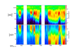
MMS1 FPI ion spectra and PAD on October 16, 2015

To generate angle-angle plots from the FPI ion distribution functions at a specific time:
<syntaxhighlight lang="idl"> MMS> mms_fpi_ang_ang, '2015-10-16/13:07:30', species='i', data_rate='brst'
</syntaxhighlight>


FPI 2D Slices
Examples
Basic 2D Slices
Load the FPI ion distribution data:
<syntaxhighlight lang="idl">
MMS> mms_load_fpi, data_rate='brst', datatype='dis-dist', probe=1, trange=['2015-10-16/13:06', '2015-10-16/13:07']
</syntaxhighlight>
Reformat the data for plotting using spd_slice2d:
<syntaxhighlight lang="idl">
MMS> dist = mms_get_dist('mms1_dis_dist_brst', trange=['2015-10-16/13:06', '2015-10-16/13:07'])
MMS> slice = spd_slice2d(dist, time='2015-10-16/13:06') ;3D interpolation
</syntaxhighlight>
Now plot the slice:
<syntaxhighlight lang="idl">
MMS> spd_slice2d_plot, slice
</syntaxhighlight>
-
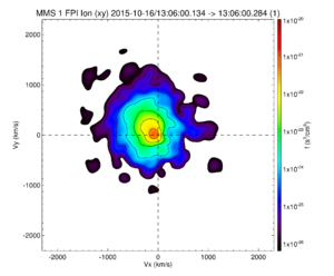
MMS1 FPI ion 2D velocity distribution slice at 13:06UT on October 16, 2015

Visualizing 3D Distribution Functions
SPEDAS can also be used for visualizing MMS 3D distribution functions from FPI using the ISEE3D tool, developed by the Institute for Space-Earth Environmental Research (ISEE), Nagoya University, Japan.
Load data into tplot
<syntaxhighlight lang="idl">
MMS> mms_load_fpi, probe=1, trange=['2015-10-20/05:56:30', '2015-10-20/05:56:34'], data_rate='brst', datatype='dis-dist'
</syntaxhighlight>
Load the data into standard structures
<syntaxhighlight lang="idl">
MMS> dist = mms_get_fpi_dist('mms1_dis_dist_brst' , trange=['2015-10-20/05:56:30', '2015-10-20/05:56:34'])
MMS> data = spd_dist_to_hash(dist) ;convert structures to isee_3d data model
</syntaxhighlight>
Load the magnetic field (cyan vector) and velocity (yellow vector) support data
<syntaxhighlight lang="idl">
MMS> mms_load_fgm, probe=1, trange=['2015-10-20/05:55:30', '2015-10-20/05:57:34'], level='l2'
MMS> mms_load_fpi, data_rate='brst', datatype='dis-moms', probe=1, trange=['2015-10-20/05:56:30', '2015-10-20/05:56:34']
</syntaxhighlight>
Once the GUI is opened, select PSD from Units menu
<syntaxhighlight lang="idl">
MMS> isee_3d, data=data, trange=['2015-10-20/05:56:30', '2015-10-20/05:56:34'], bfield='mms1_fgm_b_gse_srvy_l2_bvec', velocity='mms1_dis_bulkv_dbcs_brst'
</syntaxhighlight>
-
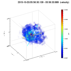
MMS1 FPI ion 3D velocity distribution at 5:56:30UT on October 20, 2015
